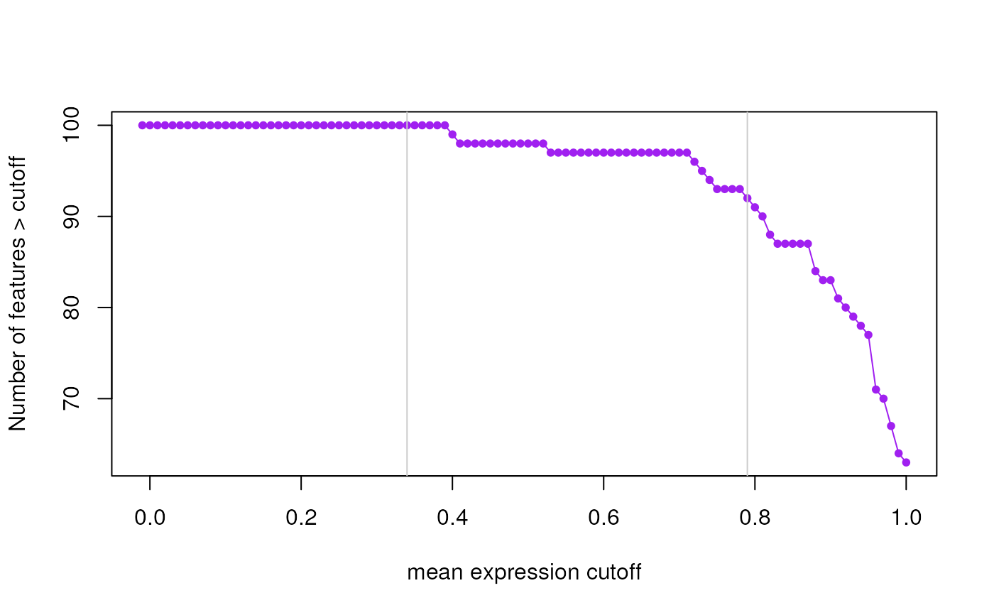
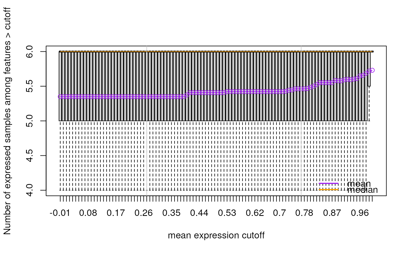
This function finds expression cutoffs based on estimating the second breakpoint using segmented applied to two curves. The first curve is the number of features passing the cutoff assuming an initial large drop, an intermediate section with moderate drop, and then a stable tail. The second curve is the mean number of expressed samples (non-zero expression) for all genes at each given cutoff. This curve increases rapidly then has a section with a moderate increase, and finally a long tail. Using segmented we find that second breakpoint. The suggested expression cutoff returned is the average of the two suggested cutoffs.
expression_cutoff(expr, max_cut = 1, seed = NULL, n.boot = 2000, k = 2)Arguments
- expr
A matrix with the expression values with features in the rows and samples in the columns in RPKM format (typically).
exprcan be any matrix asexpression_cutoff()will work with the row means of the matrix. You'll most likely want to use a normalized expression matrix, although this function will work with any matrix.- max_cut
Maximum expression cutoff to consider. Increasing this value does then to increase the suggested cutoffs. If set to
NULL, this will be chosen automatically from 1 to 5.- seed
Set this argument for increased reproducibility of the results. This is passed to seg.control. We highly recommend specifiying this value.
- n.boot
This argument controls the stability of the suggested cutoffs. It is passed to seg.control.
- k
The number of breakpoints to consider. If you increase this value the estimated breakpoints are less stable.
Value
A two element vector with the suggested cutoffs based on the number of features expressed and the mean number of expressed samples across all features. The function also makes plots that visualize both curves and show the identified breakpoints as vertical grey lines.
Examples
## Simulate expression data. Based on the limma::lmFit() man page
sd <- 0.3 * sqrt(4 / rchisq(100, df = 4))
y <- matrix(rnorm(100 * 6, sd = sd), 100, 6)
rownames(y) <- paste("Gene", seq_len(100))
y[seq_len(2), seq_len(3) + 3] <- y[seq_len(2), seq_len(3) + 3] + 2

## Make the expression data look like RPKM values
y2 <- apply(y, 2, function(z) {
    res <- z + abs(min(z))
    res[sample(seq_len(100), 10)] <- 0
    res
})
summary(y2)
#>        V1              V2               V3               V4
#>  Min.   :0.000   Min.   :0.0000   Min.   :0.0000   Min.   :0.0000
#>  1st Qu.:0.812   1st Qu.:0.5794   1st Qu.:0.6757   1st Qu.:0.7014
#>  Median :1.061   Median :0.8119   Median :0.9338   Median :1.0135
#>  Mean   :1.002   Mean   :0.8070   Mean   :0.8705   Mean   :0.9828
#>  3rd Qu.:1.264   3rd Qu.:1.0926   3rd Qu.:1.1058   3rd Qu.:1.2464
#>  Max.   :2.472   Max.   :2.1606   Max.   :1.9088   Max.   :3.3155
#>        V5              V6
#>  Min.   :0.000   Min.   :0.000
#>  1st Qu.:1.107   1st Qu.:1.435
#>  Median :1.470   Median :1.699
#>  Mean   :1.364   Mean   :1.558
#>  3rd Qu.:1.710   3rd Qu.:1.894
#>  Max.   :3.563   Max.   :3.829

expression_cutoff(y2)


#> 2024-12-12 22:07:47.514347 the suggested expression cutoff is 0.78
#> percent_features_cut  samples_nonzero_cut
#>                 0.79                 0.77

## Or same the plots to a PDF file

pdf("test_expression_cutoff.pdf", width = 12)
expression_cutoff(y2)
#> 2024-12-12 22:07:47.648362 the suggested expression cutoff is 0.78
#> percent_features_cut  samples_nonzero_cut
#>                 0.79                 0.77
dev.off()
#> pdf
#>   2

## View the pdf with the following code
utils::browseURL("test_expression_cutoff.pdf")