Lessons Learned Applying Tangram on Visium Data
By Nick Eagles
We’ve recently been interested in exploring the (largely python-based) tools others have published to process spatial transcriptomics data for various end goals. A common goal is to integrate data from platforms like Visium, which provides some information about how gene expression is spatially organized, with other approaches with potentially better spatial resolution or gene throughput. In particular, we came across a paper by Biancalani, Scalia et al. presenting a tool called Tangram, and were particularly interested in a component of the tool which could map individual cells from single cell gene expression data onto the spatial voxels probed by Visium. I encourage you to check out the paper for a more detailed description of their approach, as well as the other capabilities of their software which I won’t be covering.
There’s a lot to talk about around these topics– integrating spatial gene expression data with other forms of data, installing and running external software, and much more– but this blog post will focus on data science and machine learning lessons I learned while trying to apply Tangram on some private data.
Note: I will regularly refer to the Tangram manuscript, and several conceptual points I make (especially the role of data sparsity, trusting scores of well-selected training genes, and descriptions of the mapping learned by Tangram) are inspired by or are paraphrased from the manuscript. I intend this blog post in part to discuss these ideas, for which the authors deserve credit.
Image credit: By Nevit Dilmen - Own work, CC BY-SA 3.0, https://commons.wikimedia.org/w/index.php?curid=1798693
The Initial Plan
OK, so I had read through the paper and felt I got a basic understanding of what Tangram was doing, and some concept about how it worked. Admittedly, I had to skip over some of the more technical and advanced biological details, but I felt I had enough of the context I needed to get started. We could take single cell expression data, and learn where to “place” individual cells onto the voxels containing Visium measurements. Deep learning was used to infer this mapping?
My coworkers and I got started with Tangram’s main tutorial, where we saw that Tangram trained its mapping using a subset of genes, and that the proper selection of training genes was crucial for a robust mapping. I had prepared AnnData objects for some private data, containing single cell and Visium data, as required by the tutorial, and was ready to follow along with the code. Then, I realized that none of the marker genes selected for use in the example tutorial were present in our own data.
Somewhat naively, I was ready to experiment with different gene selection approaches, and rank them by average similarity score achieved in the test genes. Other metrics might be preferable to evaluate performance (the paper makes use of “spatial correlation”), but cosine similarity by gene was readily available as output from the tangram function tg.compare_spatial_geneexp, to compare mapped and actual expression. For each gene selection method, I took the spatially-mapped single cell expression object ad_ge, and the Visium expression object ad_sp, and computed the following metrics:
df_all_genes = tg.compare_spatial_geneexp(ad_ge, ad_sp)

#  Compute average cosine similarity for test genes
np.mean(df_all_genes.score[np.logical_not(df_all_genes.is_training)])

#  Compute average cosine similarity for training genes
np.mean(df_all_genes.score[df_all_genes.is_training])
Strangely, regardless of the selection approach used, I achieved training and test scores around 0.9 and 0.16, respectively, of course with some variation. Even for the example tutorial’s data and gene set, I achieved scores with a similarly large performance gap. What was going on here?
I more carefully reviewed the paper, and thought some more.
The Importance of Understanding your Data
As was well described in the manuscript, sparsity of gene expression, especially in the spatial data, could negatively impact similarity scores. In a particularly extreme hypothetical case, we might have a gene expressed somewhat in many cells, but whose expression in the spatial data is nonzero in only a few voxels. No matter the arrangement of cells onto voxels, it will receive a poor score owing to a relative lack of data needed to demonstrate the “true expression profile”. Figure 4f in the manuscript provides a visual display of the impact of sparsity on model performance by gene.
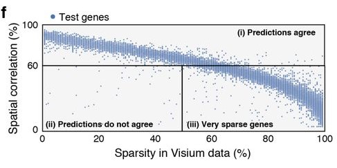
In my case, I was disproportionately selecting genes with large and diverse expression levels for training genes, and not considering expression at all when selecting test genes. We were dealing with data that fundamentally exhibited sparsity, a feature significantly influencing the model’s performance, and by ignoring it, I had created imbalanced training and test sets.
The Importance of Understanding your Model
My first instinct when observing the training/test performance gap was that serious overfitting was occurring. I was under the impression a deep neural network was used as the model which was to learn the mapping from cell to spatial voxel. However, the more I thought about it, the less it made sense that a basic arrangement task would require or even benefit from a deep neural network- this felt almost like a regression problem. Would features could a neural network even learn to solve a problem like this?
I dug deeper into the methods of the paper, and discovered the model at hand was simply a matrix, assigning probabilities for each cell to each spatial voxel. These probabilities were “directly” optimized by gradient descent to maximize a similarity score (cosine similarity) between assigned and observed gene expression levels. I made an assumption perhaps based on the title of the manuscript- but the reality was that a very “shallow”, relatively simple model was being used. In this sense, we should already be less afraid about the potential of overfitting.
Thinking more about the task Tangram’s model was learning to perform, I found it more helpful to consider the single cell- spatial mapping to be a complete jigsaw puzzle, and cells to be pieces (yes, I know the whole purpose of the name “Tangram” is as a similar metaphor). Well– imagine these pieces could hypothetically fit together in any arrangement so long as the complete picture’s shape was fixed. In this metaphor, using carefully selected training genes would be like erasing small, uninformative parts of the image on each puzzle piece. When we complete the puzzle, we will see the underlying big picture fairly well. Then, we wouldn’t particularly be worried that the erased segments might contradict what we already have in place, since we already have solid visual evidence our arrangement is good. Analogously, provided our training genes are well-selected, good training scores can give us confidence a robust mapping was found, in which we can trust test genes to be well-placed.
Takeaways
- consider the nature of your data when interpreting results, such as performance of a model on subsets of this data
- take time to understand your model, so that you can understand how to interpret its performance
- some papers need more than a brief skim :)