R 101
HAPPY HOLIDAYS!!!🎉⛄🎆🍾❄
In the spirit of the coming new year and new beginnings, we created a tutorial for getting started or restarted with R. If you are new to R or have dabbled in R but haven’t used it much recently, then this post is for you. We will focus on data classes and types, as well as data wrangling, and we will provide basic statistics and basic plotting examples using real data. Enjoy!
By C.Wright
As with most programming tutorials, let’s start with a good’ol “Hello World”.
1) First Command
print("Hello World")## [1] "Hello World"2) Install and Load Packages and Data
Now we need some data. Packages are collections of functions and/or data. There are published packages that you can use from the community such as these two packages, or you can make your own package for your own private use.
install.packages("babynames")
install.packages("titanic")
Now that we have installed the packages, we need to load them.
library("babynames")
library("titanic")
Each installation of R comes with quite a bit of data! Now we want to load the “quake” data - there are lots of other options.
data("quakes")
data() #this will list all of the datasets available
3) Assigning Objects
Objects can be many different things ranging from a simple number to a giant matrix, but they refer to things that you can manipulate in R.
myString <- "Hello World" #notice how we need "" around words, aka strings
myString #take a look at myString
## [1] "Hello World"A <- 14 #now we do not need "" around numbers
A #take a look at A## [1] 14A = 5 #can also use the equal sign to assign objects
A #notice how A has changed## [1] 54) Assigning Objects with Multiple Elements
Now lets assign a more complex object
height <- c(5.5, 4.5, 5, 5.6, 5.8, 5.2, 6, 6.2, 5.9, 5.8, 6, 5.9) #this is called a vector
colors_to_use <- c("red", "blue")# a vector of strings
5) Classes
There are a variety of different object classes. We can use the function class() to tell us what class an object belongs to.
class(height) #this is a numeric vector## [1] "numeric"class(colors_to_use) #this is a character vector## [1] "character"heightdf<-data.frame(height, gender =c("F", "F", "F", "F", "F", "F", "M", "M", "M", "M", "M", "M"))
heightdf #take a look at the dataframe## height gender
## 1 5.5 F
## 2 4.5 F
## 3 5.0 F
## 4 5.6 F
## 5 5.8 F
## 6 5.2 F
## 7 6.0 M
## 8 6.2 M
## 9 5.9 M
## 10 5.8 M
## 11 6.0 M
## 12 5.9 Mclass(heightdf) #check the class## [1] "data.frame"heightdf$height # we can refer to indivdual columns based on the column name## [1] 5.5 4.5 5.0 5.6 5.8 5.2 6.0 6.2 5.9 5.8 6.0 5.9class(heightdf$gender)#here we see a factor(categorical variable - stored in R as with integer levels## [1] "factor"logical_variable<-height == heightdf$height #this shows that all the elements in the height column of the heightdf dataframe are equivalent to those of the height vector
class(logical_variable)## [1] "logical"matrix_variable <- matrix(height, nrow = 2, ncol = 3)#now we will make a matrix
matrix_variable #take a look at the matrix## [,1] [,2] [,3]
## [1,] 5.5 5.0 5.8
## [2,] 4.5 5.6 5.2class(matrix_variable)## [1] "matrix"6) Subsetting Data
Now that we can assign or instantiate objects, let’s try to look at or manipulate specific parts of more complex objects.
Lets create an object of male heights by grabbing rows from heightdf.
maleIndex<-which(heightdf$gender == "M") #lets try subsetting just the male data out of the heightdf - first we need to determine which rows of the dataframe are male
maleIndex # this is now just a list of rows
## [1] 7 8 9 10 11 12heightmale<-heightdf[maleIndex,] #now we will use the brackets to grab these rows - we use the comma to indicate that we want rows not columns
heightmale # now this is just the males## height gender
## 7 6.0 M
## 8 6.2 M
## 9 5.9 M
## 10 5.8 M
## 11 6.0 M
## 12 5.9 MHere is another way using a package called dpylr:
install.packages("dplyr")Here we are creating an object of height data for males over 6 feet.
library(dplyr) #load a useful package for subsetting data##
## Attaching package: 'dplyr'## The following objects are masked from 'package:stats':
##
## filter, lag## The following objects are masked from 'package:base':
##
## intersect, setdiff, setequal, union#heightmale_over6feet <- dplyr::subset(heightdf, gender =="M" & height >=6)#need to use column names to describe what we want to pull out of our data
heightmale_over6feet <- subset(heightdf, gender =="M" & height >=6)#need to use column names to describe what we want to pull out of our data
heightmale_over6feet#now we just have the males 6 feet or over## height gender
## 7 6.0 M
## 8 6.2 M
## 11 6.0 MNow let’s create an object by grabbing part of an object based on its columns.
gender1<-heightdf[2]#notice how here we use the brackets but no comma
gender1
## gender
## 1 F
## 2 F
## 3 F
## 4 F
## 5 F
## 6 F
## 7 M
## 8 M
## 9 M
## 10 M
## 11 M
## 12 Mgender2<-heightdf$gender#this does the same thing #notice this way we loose the data architecture - no longer a dataframe
gender2## [1] F F F F F F M M M M M M
## Levels: F Mgender2<-data.frame(gender =heightdf$gender)# this however stays as a dataframe
gender2## gender
## 1 F
## 2 F
## 3 F
## 4 F
## 5 F
## 6 F
## 7 M
## 8 M
## 9 M
## 10 M
## 11 M
## 12 Mgenderindex<- which(colnames(heightdf) == "gender") #now wwe will use which() to select columns named gender
genderindex## [1] 2gender3 <-heightdf[genderindex]#now we will use the brackets to grab just this column
gender3## gender
## 1 F
## 2 F
## 3 F
## 4 F
## 5 F
## 6 F
## 7 M
## 8 M
## 9 M
## 10 M
## 11 M
## 12 Midentical(gender1, gender2)#lets see if they are identical - this is a helpful function - can only compare two variables at a time## [1] TRUEgender1==gender2 # are they the same? should say true if they are## gender
## [1,] TRUE
## [2,] TRUE
## [3,] TRUE
## [4,] TRUE
## [5,] TRUE
## [6,] TRUE
## [7,] TRUE
## [8,] TRUE
## [9,] TRUE
## [10,] TRUE
## [11,] TRUE
## [12,] TRUEgender2==gender3 # are they the same? should say true if they are## gender
## [1,] TRUE
## [2,] TRUE
## [3,] TRUE
## [4,] TRUE
## [5,] TRUE
## [6,] TRUE
## [7,] TRUE
## [8,] TRUE
## [9,] TRUE
## [10,] TRUE
## [11,] TRUE
## [12,] TRUENow let’s try to look at/grab specific values.
height2<-c(6, 5.5, 6, 6, 6, 6, 4.3) #6 and 5.5 are in our orignal height vector but not 4.3
which(height %in% height2) # what of our orignial data is also found in height2
## [1] 1 7 11heightdf[which(height %in% height2),] # here we skipped making another variable for the index## height gender
## 1 5.5 F
## 7 6.0 M
## 11 6.0 M#we can also use a function clalled grep
wanted_heights_index<-grep(5.9, heightdf$height)
heightdf[wanted_heights_index,] #now we just have the samples who are 5.9## height gender
## 9 5.9 M
## 12 5.9 M#say we want to know the value of an element at a particular location
heightdf$height[2] #second value in the height column## [1] 4.5heightdf$height[1:3]# first three valeus in the height column## [1] 5.5 4.5 5.0This allows you to grab random data points.
sample(heightdf$height, 2)#takes a random sample from a vector of the specified number of elements## [1] 5.5 5.9sample.int(1000999, 2)#takes a random sample from 1 to the first whole number specified. Thue number of random values to output is given by the second number.## [1] 161093 4300207) Plotting Data
Now let’s try plotting some data and perform some statistical tests.
boxplot(heightdf$height~heightdf$gender)#simple boxplot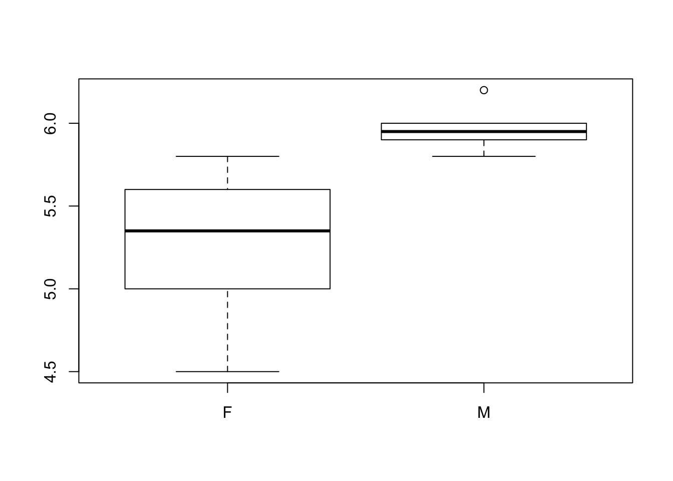
#lets make a fancy boxplot
boxplot(heightdf$height~heightdf$gender, col = c("red", "blue"), ylab = "Height", xlab = "Gender", main = "Relationship of gender and height", cex.lab =2, cex.main = 2, cex.axis = 1.3, par(mar=c(5, 5, 5, 5)))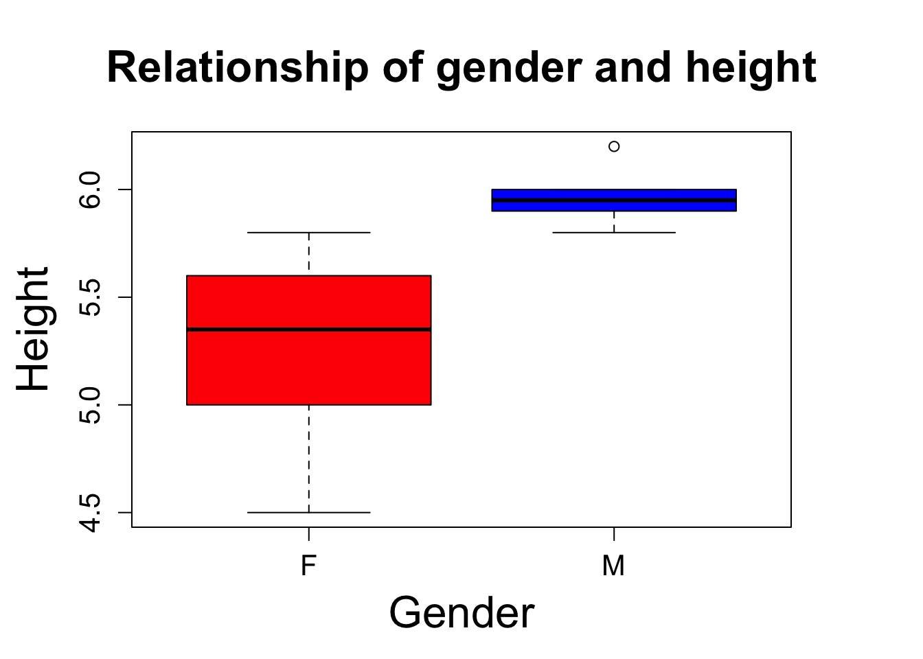
hist(heightdf$height)#histogram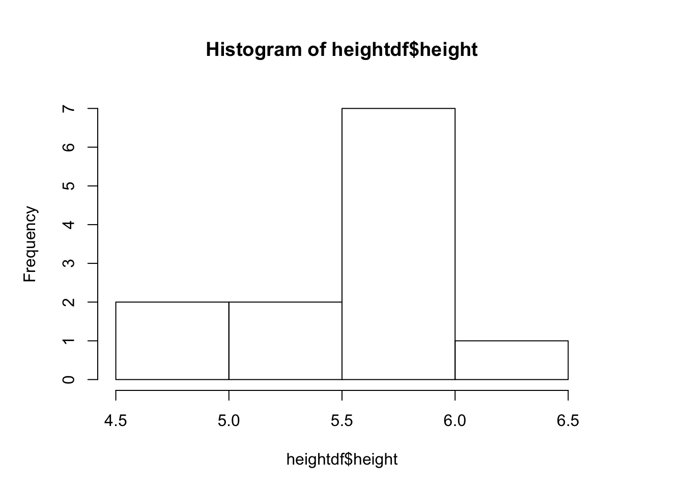
heightdf$age <-c(20, 30, 15, 20, 40, 14, 35, 40, 17, 16, 25, 16)##adding another variable to a dataframe
plot(heightdf$height)#one variable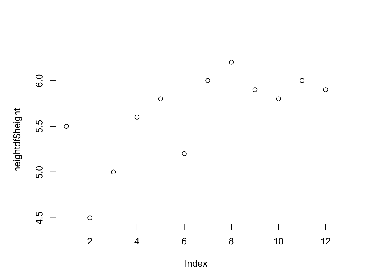
plot(y=heightdf$height, x=heightdf$age)#scatterplot of 2 variables
height_age<-lm(heightdf$height~heightdf$age)#perform a regression on the data - evaluate height and age relationship
summary(height_age)#shows the stats results from the regression
##
## Call:
## lm(formula = heightdf$height ~ heightdf$age)
##
## Residuals:
## Min 1Q Median 3Q Max
## -1.1999 -0.1154 0.1348 0.3634 0.3943
##
## Coefficients:
## Estimate Std. Error t value Pr(>|t|)
## (Intercept) 5.28384 0.39367 13.422 1.01e-07 ***
## heightdf$age 0.01387 0.01527 0.908 0.385
## ---
## Signif. codes: 0 '***' 0.001 '**' 0.01 '*' 0.05 '.' 0.1 ' ' 1
##
## Residual standard error: 0.4973 on 10 degrees of freedom
## Multiple R-squared: 0.07616, Adjusted R-squared: -0.01622
## F-statistic: 0.8244 on 1 and 10 DF, p-value: 0.3853abline(height_age)#add regression line to plot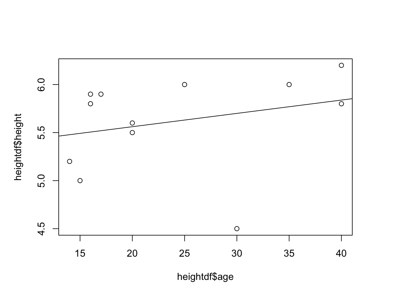
cor.test(y=heightdf$height, x=heightdf$age)#shows the same p value when performing a correlation test##
## Pearson's product-moment correlation
##
## data: heightdf$age and heightdf$height
## t = 0.90797, df = 10, p-value = 0.3853
## alternative hypothesis: true correlation is not equal to 0
## 95 percent confidence interval:
## -0.3539944 0.7336745
## sample estimates:
## cor
## 0.27597348) More Statistical Tests
t.test(heightdf$height~heightdf$gender)#try a t test between male height and female height - this is significant!##
## Welch Two Sample t-test
##
## data: heightdf$height by heightdf$gender
## t = -3.4903, df = 5.8325, p-value = 0.01359
## alternative hypothesis: true difference in means is not equal to 0
## 95 percent confidence interval:
## -1.194177 -0.205823
## sample estimates:
## mean in group F mean in group M
## 5.266667 5.966667#if p<0.05 it is generally considered significant
fit <-aov(heightdf$height~heightdf$gender + heightdf$age)#now lets perform an anova or multiple regression
summary(fit)# here are the results## Df Sum Sq Mean Sq F value Pr(>F)
## heightdf$gender 1 1.4700 1.4700 12.167 0.00685 **
## heightdf$age 1 0.1193 0.1193 0.987 0.34638
## Residuals 9 1.0874 0.1208
## ---
## Signif. codes: 0 '***' 0.001 '**' 0.01 '*' 0.05 '.' 0.1 ' ' 1anova(fit)# same results## Analysis of Variance Table
##
## Response: heightdf$height
## Df Sum Sq Mean Sq F value Pr(>F)
## heightdf$gender 1 1.47000 1.47000 12.1668 0.006851 **
## heightdf$age 1 0.11928 0.11928 0.9872 0.346383
## Residuals 9 1.08739 0.12082
## ---
## Signif. codes: 0 '***' 0.001 '**' 0.01 '*' 0.05 '.' 0.1 ' ' 1fit <-lm(heightdf$height~heightdf$gender + heightdf$age)# performing as multiple regression
summary(fit) #gives the same result as above - this is an anova but the results are presented differently##
## Call:
## lm(formula = heightdf$height ~ heightdf$gender + heightdf$age)
##
## Residuals:
## Min 1Q Median 3Q Max
## -0.83944 -0.07318 0.02918 0.12062 0.36706
##
## Coefficients:
## Estimate Std. Error t value Pr(>|t|)
## (Intercept) 5.01995 0.28600 17.552 2.86e-08 ***
## heightdf$genderM 0.68225 0.20148 3.386 0.00805 **
## heightdf$age 0.01065 0.01072 0.994 0.34638
## ---
## Signif. codes: 0 '***' 0.001 '**' 0.01 '*' 0.05 '.' 0.1 ' ' 1
##
## Residual standard error: 0.3476 on 9 degrees of freedom
## Multiple R-squared: 0.5938, Adjusted R-squared: 0.5035
## F-statistic: 6.577 on 2 and 9 DF, p-value: 0.01736anova(fit)#also gives the same result## Analysis of Variance Table
##
## Response: heightdf$height
## Df Sum Sq Mean Sq F value Pr(>F)
## heightdf$gender 1 1.47000 1.47000 12.1668 0.006851 **
## heightdf$age 1 0.11928 0.11928 0.9872 0.346383
## Residuals 9 1.08739 0.12082
## ---
## Signif. codes: 0 '***' 0.001 '**' 0.01 '*' 0.05 '.' 0.1 ' ' 1Let’s do a more classic anova - using a categorical variable with more than two categories.
heightdf$country <-c("British", "French", "British", "Dutch", "Dutch", "French", "Dutch", "Dutch", "British", "French", "British", "French")
fit <-aov(heightdf$height~heightdf$gender + heightdf$age + heightdf$country)
summary(fit)
## Df Sum Sq Mean Sq F value Pr(>F)
## heightdf$gender 1 1.4700 1.4700 19.157 0.00325 **
## heightdf$age 1 0.1193 0.1193 1.554 0.25258
## heightdf$country 2 0.5503 0.2751 3.586 0.08471 .
## Residuals 7 0.5371 0.0767
## ---
## Signif. codes: 0 '***' 0.001 '**' 0.01 '*' 0.05 '.' 0.1 ' ' 1fit <-aov(heightdf$height~ heightdf$country)
summary(fit)## Df Sum Sq Mean Sq F value Pr(>F)
## heightdf$country 2 0.6067 0.3033 1.319 0.315
## Residuals 9 2.0700 0.2300anova(fit)# we see the results of country but not each country## Analysis of Variance Table
##
## Response: heightdf$height
## Df Sum Sq Mean Sq F value Pr(>F)
## heightdf$country 2 0.60667 0.30333 1.3188 0.3146
## Residuals 9 2.07000 0.23000TukeyHSD(fit)# this is how we get these results - none are significant## Tukey multiple comparisons of means
## 95% family-wise confidence level
##
## Fit: aov(formula = heightdf$height ~ heightdf$country)
##
## $`heightdf$country`
## diff lwr upr p adj
## Dutch-British 0.30 -0.6468152 1.2468152 0.6627841
## French-British -0.25 -1.1968152 0.6968152 0.7484769
## French-Dutch -0.55 -1.4968152 0.3968152 0.2860337fit <-lm(heightdf$height~heightdf$gender + heightdf$age + heightdf$country)
summary(fit) #gives the same result as above - this is an anova just different output##
## Call:
## lm(formula = heightdf$height ~ heightdf$gender + heightdf$age +
## heightdf$country)
##
## Residuals:
## Min 1Q Median 3Q Max
## -0.36474 -0.13454 0.03405 0.15333 0.33097
##
## Coefficients:
## Estimate Std. Error t value Pr(>|t|)
## (Intercept) 5.46051 0.28225 19.346 2.46e-07 ***
## heightdf$genderM 0.71905 0.16131 4.458 0.00294 **
## heightdf$age -0.01143 0.01263 -0.905 0.39547
## heightdf$countryDutch 0.46574 0.26813 1.737 0.12596
## heightdf$countryFrench -0.25286 0.19590 -1.291 0.23778
## ---
## Signif. codes: 0 '***' 0.001 '**' 0.01 '*' 0.05 '.' 0.1 ' ' 1
##
## Residual standard error: 0.277 on 7 degrees of freedom
## Multiple R-squared: 0.7993, Adjusted R-squared: 0.6847
## F-statistic: 6.971 on 4 and 7 DF, p-value: 0.01375Lets use some real data!
Baby Name Data
This is a very fun package to check out. If you have ever wondered about the popularity of your name or someone that you know, you will find this very interesting. I also have some friends who have used it to help them name their child.
#recall that we installed and loaded this data earlier
head(babynames)#this is a special data type called a tibble - it is basically a fancy dataframe
## # A tibble: 6 x 5
## year sex name n prop
## <dbl> <chr> <chr> <int> <dbl>
## 1 1880. F Mary 7065 0.0724
## 2 1880. F Anna 2604 0.0267
## 3 1880. F Emma 2003 0.0205
## 4 1880. F Elizabeth 1939 0.0199
## 5 1880. F Minnie 1746 0.0179
## 6 1880. F Margaret 1578 0.0162tail(babynames)# we can see the data goes up to 2015## # A tibble: 6 x 5
## year sex name n prop
## <dbl> <chr> <chr> <int> <dbl>
## 1 2015. M Zyah 5 0.00000247
## 2 2015. M Zykell 5 0.00000247
## 3 2015. M Zyking 5 0.00000247
## 4 2015. M Zykir 5 0.00000247
## 5 2015. M Zyrus 5 0.00000247
## 6 2015. M Zyus 5 0.00000247#how many unique baby names are there?
length(unique(babynames$name))# that's a lot of baby names!## [1] 95025#check to see if your name is included
grep("Bob", unique(babynames$name))#looks like bob is in there## [1] 1148 2502 4948 6510 6573 6999 9443 10761 13598 13794 18059
## [12] 18701 19278 19812 20116 20921 22002 23289 26242 27453 30231 34262
## [23] 35357 37057 37702 38171 41808 42382 43247 44135 44778 46568 50097#Let's look at the values
babynames$name [grep("Bob", unique(babynames$name))] # this is a vector so we don't need to specify rows with a comma## [1] "Scott" "Tessie" "Sadye" "Una" "Philomena"
## [6] "Belva" "Rufus" "Dovie" "Janette" "Mammie"
## [11] "Melinda" "Honor" "Arch" "Denis" "Orrie"
## [16] "Floyd" "Al" "Selina" "Clora" "Elvin"
## [21] "Lafayette" "Lovie" "Armilda" "Nola" "Icy"
## [26] "Mahalia" "Gordon" "Seth" "Claudia" "Glada"
## [31] "Floyd" "Theodora" "Vella"# oops! this didn't work. why? because were aren't subsetting with an index derived from the data
unique(babynames$name) [grep("Bob", unique(babynames$name))] # here we go## [1] "Bob" "Bobbie" "Bobby" "Bobie" "Bobbye"
## [6] "Bobbe" "Bobette" "Bobetta" "Boby" "Bobbette"
## [11] "Bobbi" "Bobo" "Bobra" "Bobi" "Bobbee"
## [16] "Bobb" "Bobbetta" "Bobbyetta" "Bobbijo" "Bobbiejo"
## [21] "Bobbyjo" "Bobbiejean" "Bobbilynn" "Boban" "Bobijo"
## [26] "Bobbyjoe" "Bobak" "Bobbilee" "Bobbisue" "Bobbiesue"
## [31] "Boback" "Bobbylee" "Bobbielee"#now we can see all the variations of Bob in the data
Bob<- subset(babynames,babynames$name == "Bob")
#Let's see how much the name has been used in the past
plot(Bob$n~Bob$year)#Bob was popular but it isn't anymore 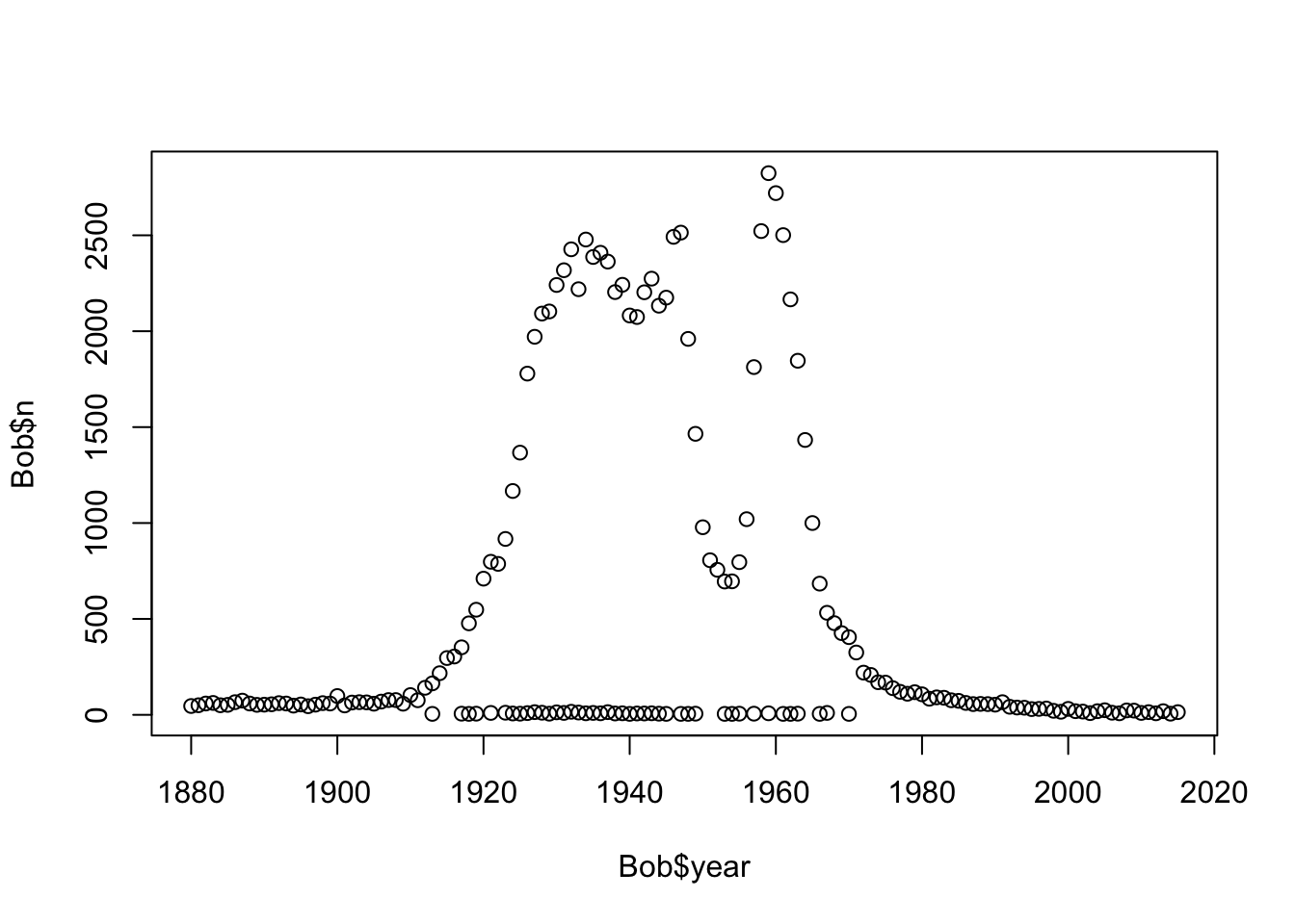
#what is the line of samples at the bottom?
plot(Bob$n~Bob$year, col= c("red", "blue")[as.factor(Bob$sex)]) 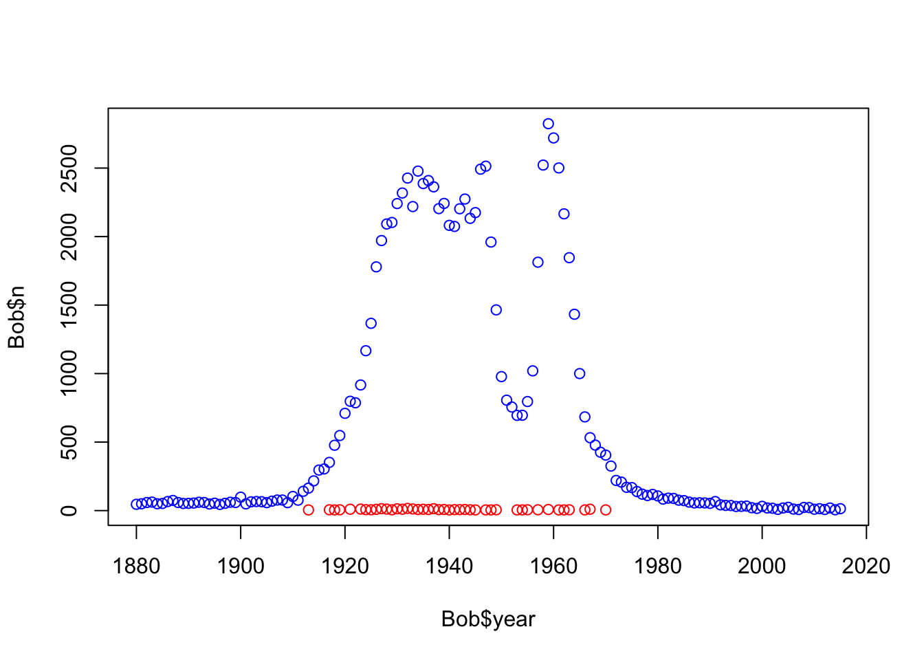
#looks like most people named Bob were male, the line of samples at the bottom are females
#lets try another name
Lori<- subset(babynames,babynames$name == "Lori")
plot(Lori$n~Lori$year, col= c("red", "blue")[as.factor(Lori$sex)])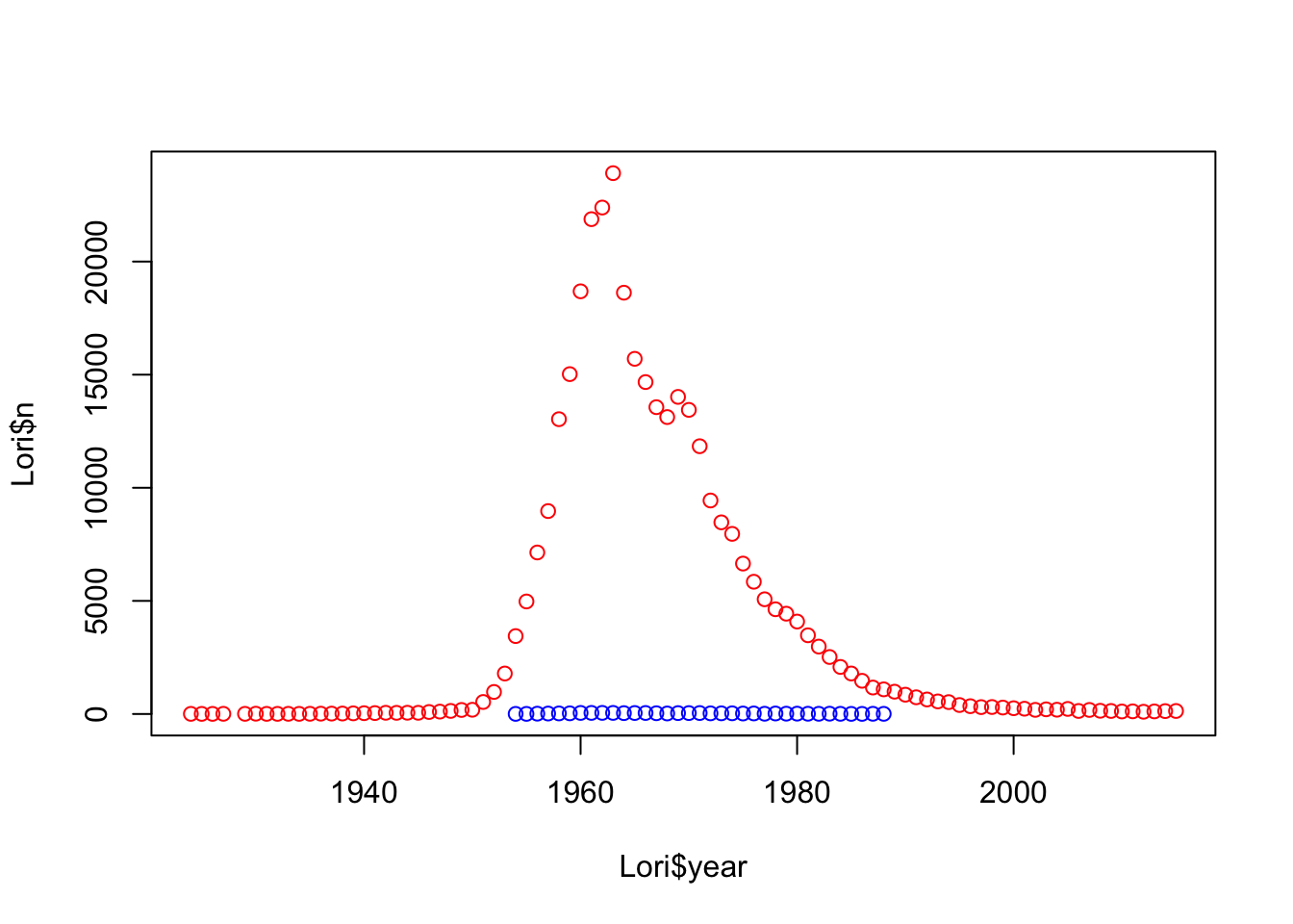
Lori_M<- subset(babynames,name == "Lori" & sex == "M")#lets look at when exactly some males were named Lori
head(Lori_M)
## # A tibble: 6 x 5
## year sex name n prop
## <dbl> <chr> <chr> <int> <dbl>
## 1 1954. M Lori 5 0.00000242
## 2 1955. M Lori 5 0.00000239
## 3 1956. M Lori 14 0.00000653
## 4 1957. M Lori 20 0.00000914
## 5 1958. M Lori 25 0.0000116
## 6 1959. M Lori 29 0.0000134# lets see how many samples are present for each year in the data
table(babynames$year)# so there are 2000 samples from 1880 and 1935 samples from 1881##
## 1880 1881 1882 1883 1884 1885 1886 1887 1888 1889 1890 1891
## 2000 1935 2127 2084 2297 2294 2392 2373 2651 2590 2695 2660
## 1892 1893 1894 1895 1896 1897 1898 1899 1900 1901 1902 1903
## 2921 2831 2941 3049 3091 3028 3264 3042 3731 3153 3362 3389
## 1904 1905 1906 1907 1908 1909 1910 1911 1912 1913 1914 1915
## 3561 3655 3633 3948 4018 4227 4629 4867 6351 6967 7964 9358
## 1916 1917 1918 1919 1920 1921 1922 1923 1924 1925 1926 1927
## 9696 9915 10401 10368 10756 10856 10757 10641 10869 10641 10460 10405
## 1928 1929 1930 1931 1932 1933 1934 1935 1936 1937 1938 1939
## 10159 9816 9788 9293 9383 9011 9181 9035 8893 8945 9030 8919
## 1940 1941 1942 1943 1944 1945 1946 1947 1948 1949 1950 1951
## 8960 9087 9424 9405 9153 9026 9702 10370 10237 10264 10309 10460
## 1952 1953 1954 1955 1956 1957 1958 1959 1960 1961 1962 1963
## 10654 10831 10963 11114 11339 11564 11521 11771 11924 12178 12206 12278
## 1964 1965 1966 1967 1968 1969 1970 1971 1972 1973 1974 1975
## 12394 11953 12148 12400 12930 13746 14782 15291 15414 15676 16243 16934
## 1976 1977 1978 1979 1980 1981 1982 1983 1984 1985 1986 1987
## 17395 18171 18224 19032 19439 19470 19680 19398 19501 20076 20642 21399
## 1988 1989 1990 1991 1992 1993 1994 1995 1996 1997 1998 1999
## 22360 23769 24715 25104 25421 25959 25998 26080 26420 26966 27894 28546
## 2000 2001 2002 2003 2004 2005 2006 2007 2008 2009 2010 2011
## 29764 30264 30559 31179 32040 32539 34073 34941 35051 34689 34050 33880
## 2012 2013 2014 2015
## 33697 33229 33176 32952# Ok, so more samples were included in the more recent years
hist(babynames$year)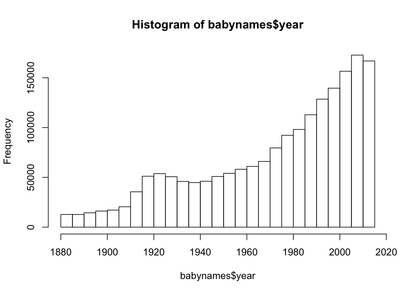
Let’s look at some other data…
Titanic Data
This package contains real data about the passengers that were aboard the Titanic.
head(Titanic) # we can see that this may be an unusal data type## [1] 0 0 35 0 0 0class(Titanic) # indeed this appears to be a table## [1] "table"dim(Titanic)## [1] 4 2 2 2dimnames(Titanic)## $Class
## [1] "1st" "2nd" "3rd" "Crew"
##
## $Sex
## [1] "Male" "Female"
##
## $Age
## [1] "Child" "Adult"
##
## $Survived
## [1] "No" "Yes"str(Titanic) # shows the structure of the data## table [1:4, 1:2, 1:2, 1:2] 0 0 35 0 0 0 17 0 118 154 ...
## - attr(*, "dimnames")=List of 4
## ..$ Class : chr [1:4] "1st" "2nd" "3rd" "Crew"
## ..$ Sex : chr [1:2] "Male" "Female"
## ..$ Age : chr [1:2] "Child" "Adult"
## ..$ Survived: chr [1:2] "No" "Yes"help("titanic_test")#this shows more information about the data
help("titanic_train")# I would assume survived is a 1
#lets see if more males or females survived
boxplot(titanic_train$Survived~titanic_train$Sex)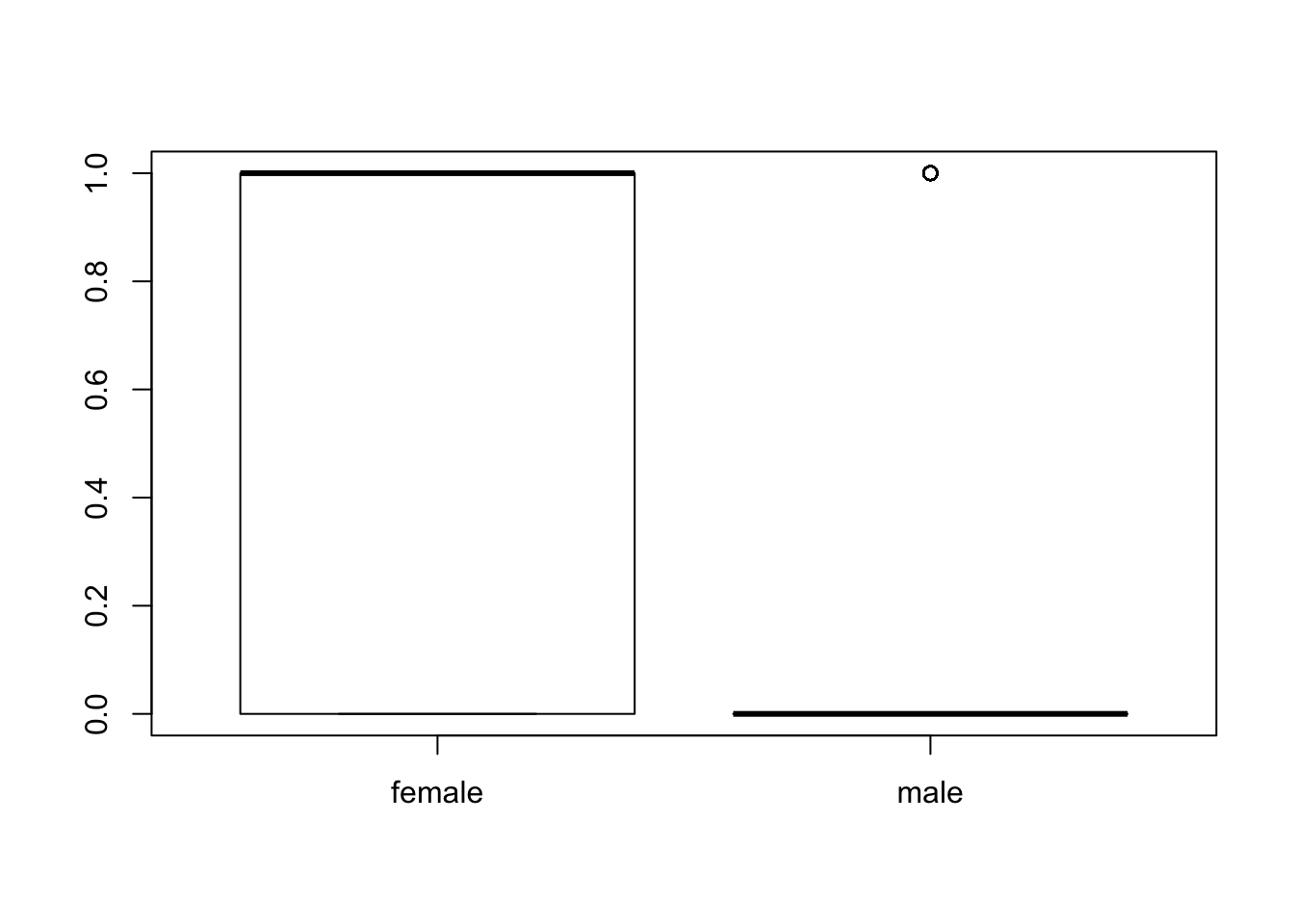
table(titanic_train$Survived,titanic_train$Sex)# it looks like males laregly did not survive##
## female male
## 0 81 468
## 1 233 109# this might be a better way to view the data - here width represents the number of samples - thus there are more males overall
mosaicplot(Sex ~ Survived, data=titanic_train) 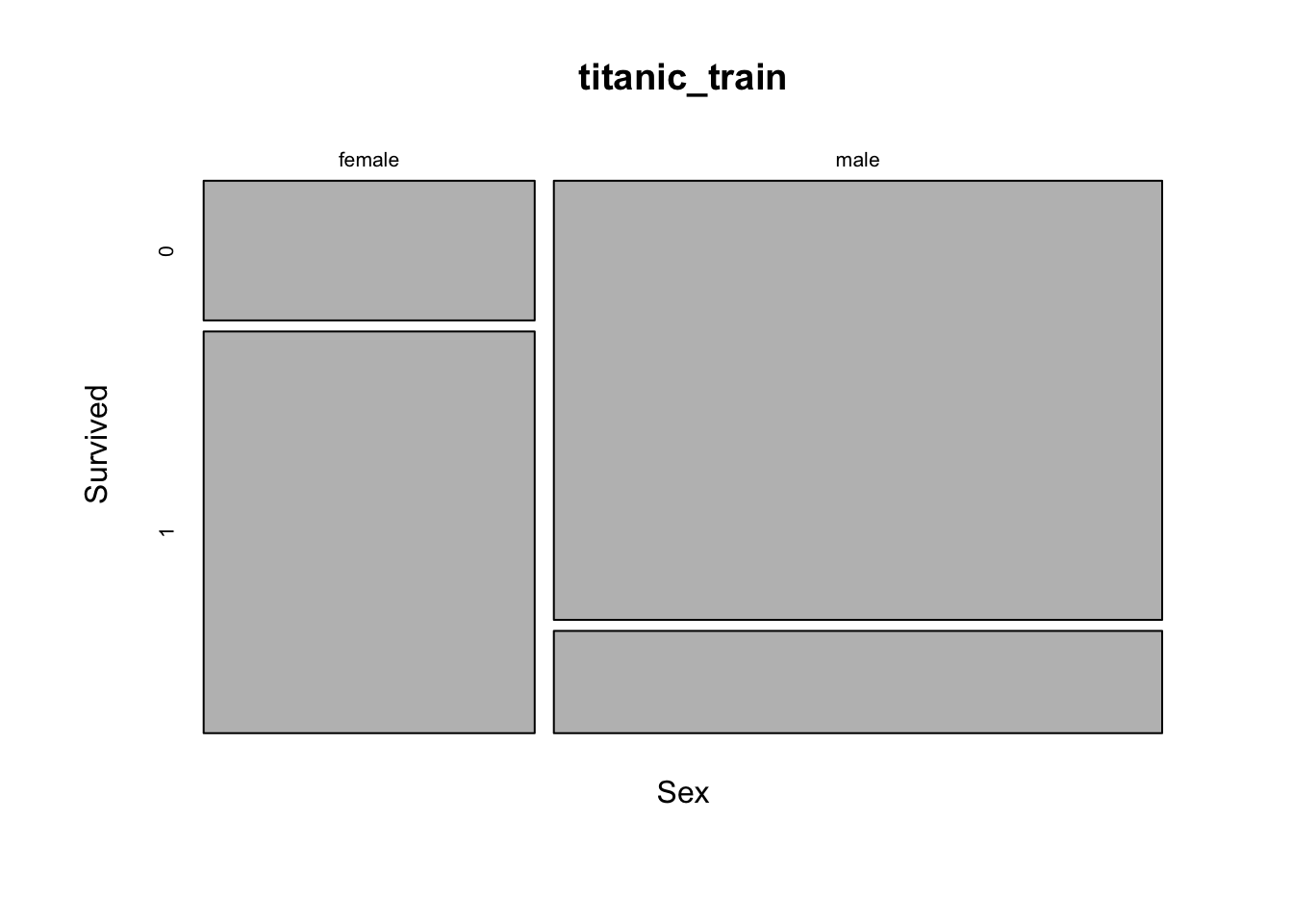
# It looks like even though there were many more males, the female passangers were much more likely to surviveHow about some more data…
Earthquake Data
Here we will scrape data (or obtain data from a website) from the USGS website about earthquake rates in different US states. See our previous post from S. Semick on scraping data from research articles for more information on how to do this.
install.packages("htmltab")
install.packages("reshape2")
library(htmltab)
library(reshape2)## Warning: package 'reshape2' was built under R version 3.4.3url<-"https://earthquake.usgs.gov/earthquakes/browse/stats.php"
eq <- htmltab(doc = url, which = 5)## No encoding supplied: defaulting to UTF-8.rownames(eq)<-eq$States
eq<-eq[-1]
head(eq)## 2010 2011 2012 2013 2014 2015
## Alabama 1 1 0 0 2 6
## Alaska 2245 1409 1166 1329 1296 1575
## Arizona 6 7 4 3 31 10
## Arkansas 15 44 4 4 1 0
## California 546 195 243 240 191 130
## Colorado 4 23 7 2 13 7eq2 <- as.data.frame(sapply(eq, function(x) as.numeric(as.character(x))))
head(eq2)## 2010 2011 2012 2013 2014 2015
## 1 1 1 0 0 2 6
## 2 2245 1409 1166 1329 1296 1575
## 3 6 7 4 3 31 10
## 4 15 44 4 4 1 0
## 5 546 195 243 240 191 130
## 6 4 23 7 2 13 7convertoChar<-function(x) as.numeric(as.character(x)) # or you could create a function to use multiple times
factor_to_fix<-as.factor(c(1,2))
class(factor_to_fix)## [1] "factor"class(trying_function<-convertoChar(x=factor_to_fix))# now the class is numeric## [1] "numeric"class(trying_function2<-convertoChar(factor_to_fix))# now the class is numeric## [1] "numeric"rownames(eq2)<-rownames(eq)
head(eq2)## 2010 2011 2012 2013 2014 2015
## Alabama 1 1 0 0 2 6
## Alaska 2245 1409 1166 1329 1296 1575
## Arizona 6 7 4 3 31 10
## Arkansas 15 44 4 4 1 0
## California 546 195 243 240 191 130
## Colorado 4 23 7 2 13 7colSums(eq2)#look at the col sums## 2010 2011 2012 2013 2014 2015
## 3026 1955 1603 1899 2628 3225colMeans(eq2)# look at the col means## 2010 2011 2012 2013 2014 2015
## 60.52 39.10 32.06 37.98 52.56 64.50rowMeans(eq2)## Alabama Alaska Arizona Arkansas California
## 1.6666667 1503.3333333 10.1666667 11.3333333 257.5000000
## Colorado Connecticut Delaware Florida Georgia
## 9.3333333 0.1666667 0.0000000 0.0000000 0.0000000
## Hawaii Idaho Illinois Indiana Iowa
## 33.3333333 15.8333333 0.8333333 0.6666667 0.0000000
## Kansas Kentucky Louisiana Maine Maryland
## 17.3333333 0.3333333 0.1666667 0.5000000 0.1666667
## Massachusetts Michigan Minnesota Mississippi Missouri
## 0.0000000 0.3333333 0.1666667 0.5000000 2.1666667
## Montana Nebraska Nevada New Hampshire New Jersey
## 14.8333333 1.0000000 85.5000000 0.1666667 0.0000000
## New Mexico New York North Carolina North Dakota Ohio
## 6.3333333 0.5000000 0.1666667 0.1666667 1.0000000
## Oklahoma Oregon Pennsylvania Rhode Island South Carolina
## 285.6666667 2.8333333 0.0000000 0.0000000 0.5000000
## South Dakota Tennessee Texas Utah Vermont
## 1.0000000 1.3333333 13.8333333 11.5000000 0.0000000
## Virginia Washington West Virginia Wisconsin Wyoming
## 2.1666667 10.0000000 0.3333333 0.0000000 84.6666667rowSums(eq2)## Alabama Alaska Arizona Arkansas California
## 10 9020 61 68 1545
## Colorado Connecticut Delaware Florida Georgia
## 56 1 0 0 0
## Hawaii Idaho Illinois Indiana Iowa
## 200 95 5 4 0
## Kansas Kentucky Louisiana Maine Maryland
## 104 2 1 3 1
## Massachusetts Michigan Minnesota Mississippi Missouri
## 0 2 1 3 13
## Montana Nebraska Nevada New Hampshire New Jersey
## 89 6 513 1 0
## New Mexico New York North Carolina North Dakota Ohio
## 38 3 1 1 6
## Oklahoma Oregon Pennsylvania Rhode Island South Carolina
## 1714 17 0 0 3
## South Dakota Tennessee Texas Utah Vermont
## 6 8 83 69 0
## Virginia Washington West Virginia Wisconsin Wyoming
## 13 60 2 0 508max(eq2)# maximum value## [1] 2245boxplot(eq2)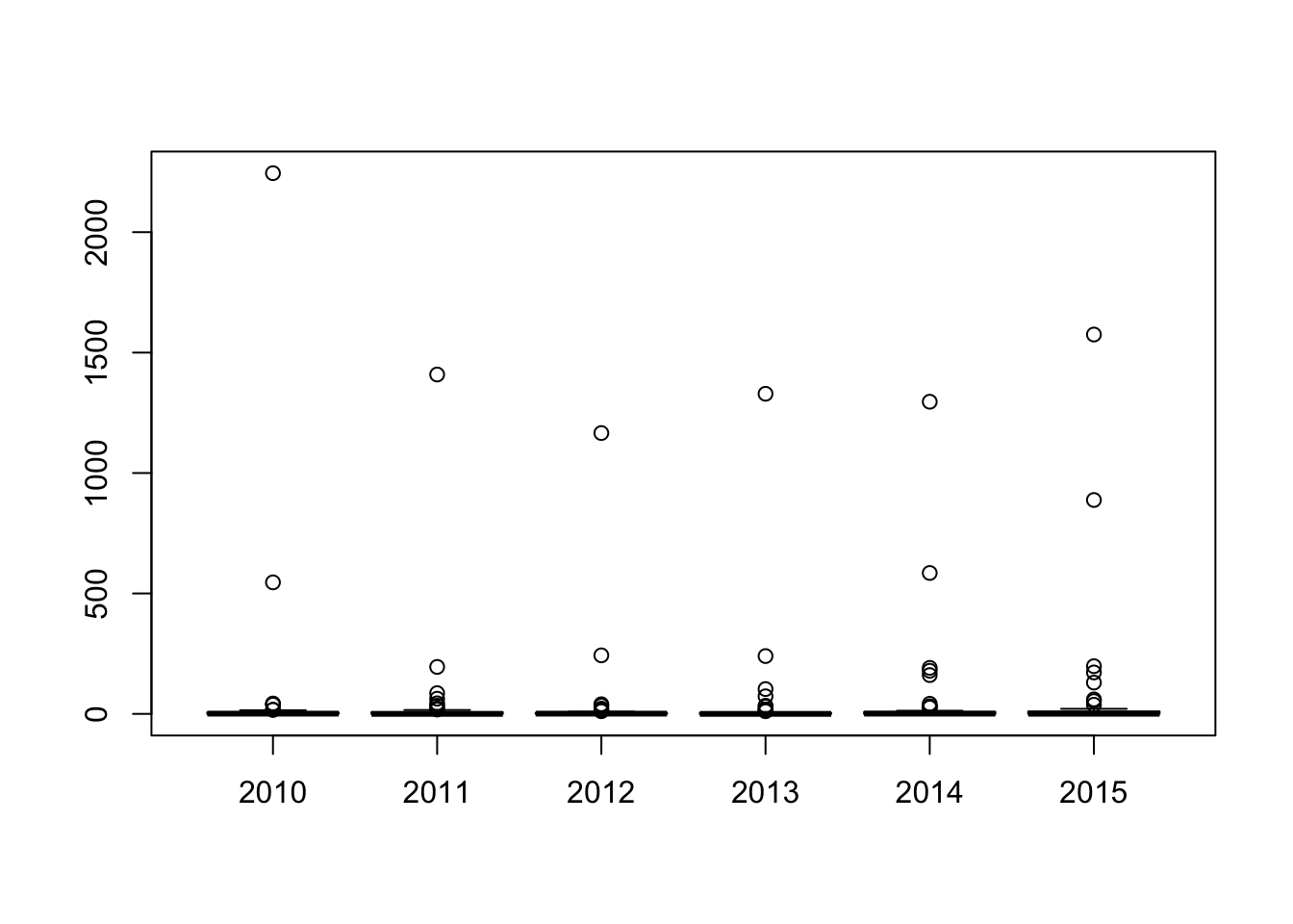
boxplot(eq2, ylim = c(0,40))# change the limit of the plot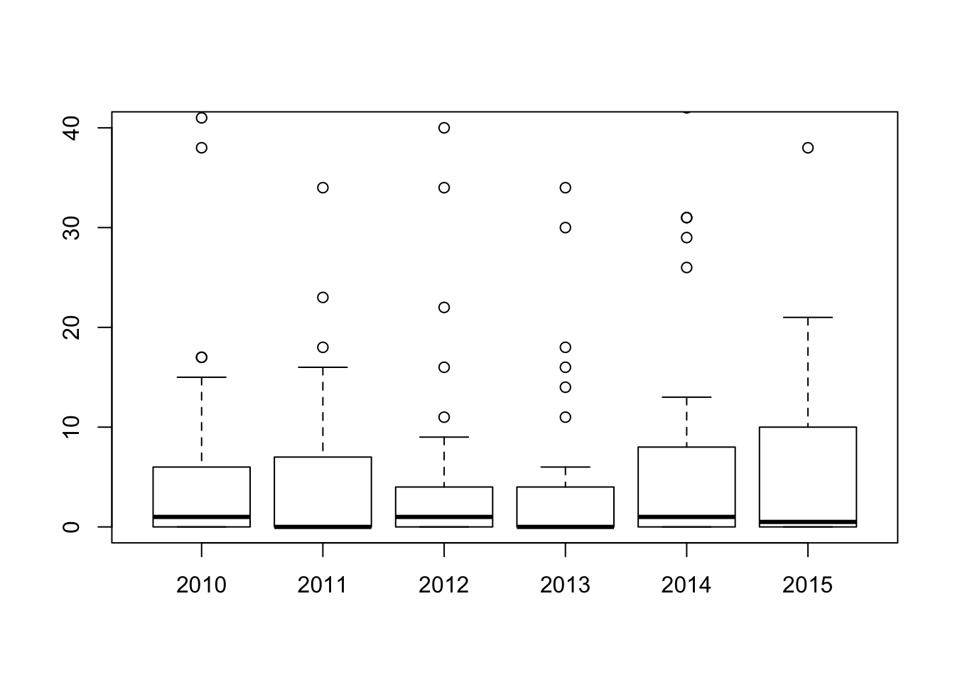
boxplot(t(eq2), ylim =c(0,2000))#flip the data using t()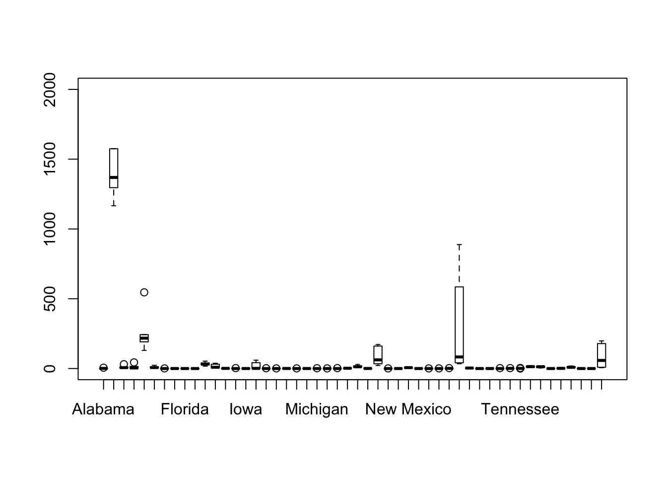
eq3<-melt(eq2)#this puts the data in long form## No id variables; using all as measure variablesnames(eq3)<-c("year", "quakes")
head(eq3)## year quakes
## 1 2010 1
## 2 2010 2245
## 3 2010 6
## 4 2010 15
## 5 2010 546
## 6 2010 4fit<-aov(eq3$quakes~eq3$year)
summary(fit)#no significant difference by year## Df Sum Sq Mean Sq F value Pr(>F)
## eq3$year 5 44161 8832 0.169 0.974
## Residuals 294 15405834 52401In addition, these are functions that the members of LIBD Rstats use often:
- head() / tail() – see the head and the tail - also check out the corner function of the jaffelab package created by LIBD Rstats founding member E. Burke
- colnames() / rownames() – see and rename columns or row names
- colMeans() / rowMeans() / colSums() / rowSums() – get means and sums of columns and rows
- dim() and length() – determine the dimensions/size of a data set – need to use length() when evaluating a vector
- ncol() / nrow() – number of columns and rows
- str() – displays the structure of an object - this is very useful with complex data structures
- unique()/duplicated() – find unique and duplicated values
- order()/sort()– order and sort your data
- gsub() – replace values
- table() – summarize your data in table format
- t.test() – perform a t test
- cor.test() – perform a correlation test
- lm() – make a linear model
- summary() – if you use the lm() output – this will give you the results
- set.seed() – allows for random permutations or random data to be the same every time your run your code
For additional help take a look at these links:
Free courses and tutorials
Community support
- https://community.rstudio.com/
- https://support.bioconductor.org/
- https://resources.rstudio.com/webinars/help-me-help-you-creating-reproducible-examples-jenny-bryan
- link helps you make examples of code errors that you need help with
Tips for help
- https://www.r-project.org/help.html
- Google! – stackoverflow, biostars
- https://www.rstudio.com/resources/cheatsheets/
Also follow our blog for more helpful posts.
Thanks for reading and have fun getting to know R!

This image came from: https://www.pinterest.com/pin/89790586304535333/
Acknowledgments
This blog post was made possible thanks to:
References
[1] C. Boettiger. knitcitations: Citations for ‘Knitr’ Markdown Files. R package version 1.0.8. 2017. URL: https://CRAN.R-project.org/package=knitcitations.
[2] G. Csárdi, R. core, H. Wickham, W. Chang, et al. sessioninfo: R Session Information. R package version 1.1.1. 2018. URL: https://CRAN.R-project.org/package=sessioninfo.
[3] A. Oleś, M. Morgan and W. Huber. BiocStyle: Standard styles for vignettes and other Bioconductor documents. R package version 2.6.1. 2017. URL: https://github.com/Bioconductor/BiocStyle.
[4] Y. Xie, A. P. Hill and A. Thomas. blogdown: Creating Websites with R Markdown. ISBN 978-0815363729. Boca Raton, Florida: Chapman and Hall/CRC, 2017. URL: https://github.com/rstudio/blogdown.
Reproducibility
## ─ Session info ───────────────────────────────────────────────────────────────────────────────────────────────────────
##  setting  value
##  version  R version 3.4.0 (2017-04-21)
##  os       macOS Sierra 10.12.6
##  system   x86_64, darwin15.6.0
##  ui       X11
##  language (EN)
##  collate  en_US.UTF-8
##  ctype    en_US.UTF-8
##  tz       America/New_York
##  date     2018-11-19
##
## ─ Packages ───────────────────────────────────────────────────────────────────────────────────────────────────────────
##  package       * version   date       lib source
##  assertthat      0.2.0     2017-04-11 [1] CRAN (R 3.4.0)
##  babynames     * 0.3.0     2017-04-14 [1] CRAN (R 3.4.0)
##  backports       1.1.2     2018-04-18 [1] Github (r-lib/backports@cee9348)
##  bibtex          0.4.2     2017-06-30 [1] CRAN (R 3.4.1)
##  bindr           0.1       2016-11-13 [1] CRAN (R 3.4.0)
##  bindrcpp        0.2       2017-06-17 [1] CRAN (R 3.4.0)
##  BiocStyle     * 2.6.1     2017-11-30 [1] Bioconductor
##  blogdown        0.5.9     2018-03-08 [1] Github (rstudio/blogdown@dc1f41c)
##  bookdown        0.7       2018-02-18 [1] CRAN (R 3.4.3)
##  cli             1.0.0     2017-11-05 [1] CRAN (R 3.4.2)
##  crayon          1.3.4     2017-09-16 [1] CRAN (R 3.4.1)
##  curl            3.2       2018-03-28 [1] CRAN (R 3.4.4)
##  digest          0.6.15    2018-01-28 [1] CRAN (R 3.4.3)
##  dplyr         * 0.7.4     2017-09-28 [1] CRAN (R 3.4.2)
##  evaluate        0.11      2018-07-17 [1] CRAN (R 3.4.4)
##  glue            1.3.0     2018-07-17 [1] CRAN (R 3.4.4)
##  htmltab       * 0.7.1     2016-12-29 [1] CRAN (R 3.4.0)
##  htmltools       0.3.6     2017-04-28 [1] CRAN (R 3.4.0)
##  httr            1.3.1     2017-08-20 [1] CRAN (R 3.4.1)
##  jsonlite        1.5       2017-06-01 [1] CRAN (R 3.4.0)
##  knitcitations * 1.0.8     2017-07-04 [1] CRAN (R 3.4.1)
##  knitr           1.20      2018-02-20 [1] CRAN (R 3.4.3)
##  lubridate       1.7.4     2018-04-11 [1] CRAN (R 3.4.4)
##  magrittr        1.5       2014-11-22 [1] CRAN (R 3.4.0)
##  pillar          1.2.1     2018-02-27 [1] CRAN (R 3.4.3)
##  pkgconfig       2.0.1     2017-03-21 [1] CRAN (R 3.4.0)
##  plyr            1.8.4     2016-06-08 [1] CRAN (R 3.4.0)
##  R6              2.2.2     2017-06-17 [1] CRAN (R 3.4.0)
##  Rcpp            0.12.16   2018-03-13 [1] CRAN (R 3.4.4)
##  RefManageR      1.2.0     2018-04-25 [1] CRAN (R 3.4.4)
##  reshape2      * 1.4.3     2017-12-11 [1] CRAN (R 3.4.3)
##  rlang           0.2.0     2018-02-20 [1] CRAN (R 3.4.3)
##  rmarkdown       1.10      2018-06-11 [1] CRAN (R 3.4.4)
##  rprojroot       1.3-2     2018-01-03 [1] CRAN (R 3.4.3)
##  sessioninfo   * 1.1.1     2018-11-05 [1] CRAN (R 3.4.4)
##  stringi         1.2.4     2018-07-20 [1] CRAN (R 3.4.4)
##  stringr         1.3.1     2018-05-10 [1] CRAN (R 3.4.4)
##  tibble          1.4.2     2018-01-22 [1] CRAN (R 3.4.3)
##  titanic       * 0.1.0     2015-08-31 [1] CRAN (R 3.4.0)
##  utf8            1.1.3     2018-01-03 [1] CRAN (R 3.4.3)
##  withr           2.1.2     2018-03-15 [1] CRAN (R 3.4.4)
##  xfun            0.3       2018-07-06 [1] CRAN (R 3.4.4)
##  XML             3.98-1.10 2018-02-19 [1] CRAN (R 3.4.3)
##  xml2            1.2.0     2018-01-24 [1] CRAN (R 3.4.3)
##  yaml            2.2.0     2018-07-25 [1] CRAN (R 3.4.4)
##
## [1] /Library/Frameworks/R.framework/Versions/3.4/Resources/library