recount3 quick start guide
Leonardo Collado-Torres
Lieber Institute for Brain Development, Johns Hopkins Medical CampusCenter for Computational Biology, Johns Hopkins Universitylcolladotor@gmail.com
1 April 2026
Source:vignettes/recount3-quickstart.Rmd
recount3-quickstart.Rmd![]()
Overview
The recount3 R/Bioconductor package is an interface to the recount3 project. recount3 provides uniformly processed RNA-seq data for hundreds of thousands of samples. The R package makes it possible to easily retrieve this data in standard Bioconductor containers, including RangedSummarizedExperiment. The sections on terminology and available data contains more detail on those subjects.
The main documentation website for all the
recount3-related projects is available at recount.bio.
Please check that website for more information about how this
R/Bioconductor package and other tools are related to each other.
Basics
Installing recount3
R is an open-source statistical environment which can be
easily modified to enhance its functionality via packages. recount3
is a R package available via the Bioconductor repository
for packages. R can be installed on any operating system
from CRAN after which you can
install recount3
by using the following commands in your R session:
if (!requireNamespace("BiocManager", quietly = TRUE)) {
    install.packages("BiocManager")
}

BiocManager::install("recount3")

## Check that you have a valid Bioconductor installation
BiocManager::valid()
You can install the development version from GitHub with:
BiocManager::install("LieberInstitute/recount3")Required knowledge
recount3 is based on many other packages and in particular in those that have implemented the infrastructure needed for dealing with RNA-seq data. A recount3 user will benefit from being familiar with SummarizedExperiment to understand the objects recount3 generates. It might also prove to be highly beneficial to check the
- DESeq2 and limma packages for performing differential expression analysis with the RangedSummarizedExperiment objects,
- DEFormats package for switching the objects to those used by other differential expression packages such as edgeR,
- derfinder package for performing annotation-agnostic differential expression analysis.
-
recount
package which provided an R/Bioconductor interface to the data in the
recount2project (Collado-Torres, Nellore, Kammers, Ellis et al., 2017; Collado-Torres, Nellore, and Jaffe, 2017).
If you are asking yourself the question “Where do I start using Bioconductor?” you might be interested in this blog post.
Asking for help
As package developers, we try to explain clearly how to use our
packages and in which order to use the functions. But R and
Bioconductor have a steep learning curve so it is critical
to learn where to ask for help. The blog post quoted above mentions some
but we would like to highlight the Bioconductor support site
as the main resource for getting help: remember to use the
recount3 tag and check the older
posts. Other alternatives are available such as creating GitHub
issues and tweeting. However, please note that if you want to receive
help you should adhere to the posting
guidelines. It is particularly critical that you provide a small
reproducible example and your session information so package developers
can track down the source of the error.
Citing recount3
We hope that recount3 will be useful for your research. Please use the following information to cite the package and the overall approach. Thank you!
## Citation info
citation("recount3")
#> To cite package 'recount3' in publications use:
#>
#>   Collado-Torres L (2026). _Explore and download data from the recount3
#>   project_. doi:10.18129/B9.bioc.recount3
#>   <https://doi.org/10.18129/B9.bioc.recount3>.
#>   https://github.com/LieberInstitute/recount3 - R package version
#>   1.21.1, <http://www.bioconductor.org/packages/recount3>.
#>
#>   Wilks C, Zheng SC, Chen FY, Charles R, Solomon B, Ling JP, Imada EL,
#>   Zhang D, Joseph L, Leek JT, Jaffe AE, Nellore A, Collado-Torres L,
#>   Hansen KD, Langmead B (2021). "recount3: summaries and queries for
#>   large-scale RNA-seq expression and splicing." _Genome Biol_.
#>   doi:10.1186/s13059-021-02533-6
#>   <https://doi.org/10.1186/s13059-021-02533-6>.
#>   <https://doi.org/10.1186/s13059-021-02533-6>.
#>
#> To see these entries in BibTeX format, use 'print(<citation>,
#> bibtex=TRUE)', 'toBibtex(.)', or set
#> 'options(citation.bibtex.max=999)'.
Quick start
After installing recount3 (Wilks, Zheng, Chen, Charles et al., 2021), we need to load the package, which will automatically load the required dependencies.
## Load recount3 R package
library("recount3")
If you have identified a study of interest and want
to access the gene level expression data, use create_rse()
as shown below. create_rse() has arguments that will allow
you to specify the annotation of interest for the given
organism, and whether you want to download gene,
exon or exon-exon junction expression
data.
## Find all available human projects
human_projects <- available_projects()
#> 2026-04-01 03:50:48.572557 caching file sra.recount_project.MD.gz.
#> 2026-04-01 03:50:48.906166 caching file gtex.recount_project.MD.gz.
#> 2026-04-01 03:50:49.186476 caching file tcga.recount_project.MD.gz.

## Find the project you are interested in,
## here we use SRP009615 as an example
proj_info <- subset(
    human_projects,
    project == "SRP009615" & project_type == "data_sources"
)

## Create a RangedSummarizedExperiment (RSE) object at the gene level
rse_gene_SRP009615 <- create_rse(proj_info)
#> 2026-04-01 03:50:52.661298 downloading and reading the metadata.
#> 2026-04-01 03:50:52.922527 caching file sra.sra.SRP009615.MD.gz.
#> 2026-04-01 03:50:53.152977 caching file sra.recount_project.SRP009615.MD.gz.
#> 2026-04-01 03:50:53.437819 caching file sra.recount_qc.SRP009615.MD.gz.
#> 2026-04-01 03:50:53.718043 caching file sra.recount_seq_qc.SRP009615.MD.gz.
#> 2026-04-01 03:50:54.017443 caching file sra.recount_pred.SRP009615.MD.gz.
#> 2026-04-01 03:50:54.07667 downloading and reading the feature information.
#> 2026-04-01 03:50:54.344145 caching file human.gene_sums.G026.gtf.gz.
#> 2026-04-01 03:50:55.396882 downloading and reading the counts: 12 samples across 63856 features.
#> 2026-04-01 03:50:55.608165 caching file sra.gene_sums.SRP009615.G026.gz.
#> 2026-04-01 03:50:55.731431 constructing the RangedSummarizedExperiment (rse) object.

## Explore that RSE object
rse_gene_SRP009615
#> class: RangedSummarizedExperiment
#> dim: 63856 12
#> metadata(8): time_created recount3_version ... annotation recount3_url
#> assays(1): raw_counts
#> rownames(63856): ENSG00000278704.1 ENSG00000277400.1 ...
#>   ENSG00000182484.15_PAR_Y ENSG00000227159.8_PAR_Y
#> rowData names(10): source type ... havana_gene tag
#> colnames(12): SRR387777 SRR387778 ... SRR389077 SRR389078
#> colData names(175): rail_id external_id ...
#>   recount_pred.curated.cell_line BigWigURL
Once you have a RSE file, you can use transform_counts()
to transform the raw coverage counts.
## Once you have your RSE object, you can transform the raw coverage
## base-pair coverage counts using transform_counts().
## For RPKM, TPM or read outputs, check the details in transform_counts().
assay(rse_gene_SRP009615, "counts") <- transform_counts(rse_gene_SRP009615)
Now you are ready to continue with downstream analysis software.
recount3 also supports accessing the BigWig raw coverage files as well as specific study or collection sample metadata. Please continue to the users guide for more detailed information.
Users guide
recount3
(Wilks, Zheng,
Chen, Charles et al., 2021) provides an interface for downloading
the recount3
raw files and building Bioconductor-friendly R objects
(Huber,
Carey, Gentleman, Anders et al., 2015;
Morgan,
Obenchain, Hester, and Pagès, 2019) that can be used with many
downstream packages. To achieve this, the raw data is organized by
study from a specific data source.
That same study can be a part of one or more
collections, which is a manually curated set of studies
with collection-specific sample metadata (see the Data
source vs collection for details). To get started with recount3,
you will need to identify the ID for the study of interest from either
human or mouse for a particular
annotation of interest. Once you have identified study,
data source or collection, and annotation, recount3
can be used to build a RangedSummarizedExperiment object
(Morgan,
Obenchain, Hester, and Pagès, 2019) for either
gene, exon or exon-exon
junction expression feature data. Furthermore, recount3
provides access to the coverage BigWig files that can be quantified for
custom set of genomic regions using megadepth.
Furthermore, snapcount
allows fast-queries for custom exon-exon junctions and other custom
input.
Available data
recount3
provides access to most of the recount3
raw files in a form that is R/Bioconductor-friendly. As a summary of
the data provided by the recount3 project (Figure
@ref(fig:recountWorkflowFig1)), the main data files provided are:
-
metadata: information about the samples in
recount3, which can come from sources such as the Sequence Read Archive as well asrecount3quality metrics. -
gene: RNA expression data quantified at the gene
annotation level. This information is provided for multiple annotations
that are organism-specific. Similar to the
recount2project, therecount3project provides counts at the base-pair coverage level (Collado-Torres, Nellore, and Jaffe, 2017). - exon: RNA expression data quantified at the exon annotation level. The data is also annotation-specific and the counts are also at the base-pair coverage level.
- exon-exon junctions: RNA expression data quantified at the exon-exon junction level. This data is annotation-agnostic (it does not depend on the annotation) and is variable across each study because different sets of exon-exon junctions are measured in each study.
- bigWig: RNA expression data in raw format at the base-pair coverage resolution. This raw data when coupled with a given annotation can be used to generate gene and exon level counts using software such as megadepth. It enables exploring the RNA expression landscape in an annotation-agnostic way.
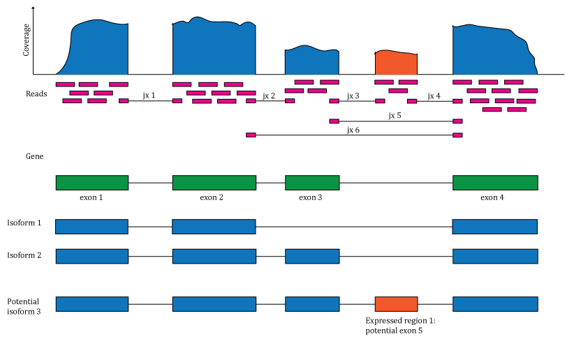
Overview of the data available in recount2 and recount3. Reads (pink boxes) aligned to the reference genome can be used to compute a base-pair coverage curve and identify exon-exon junctions (split reads). Gene and exon count matrices are generated using annotation information providing the gene (green boxes) and exon (blue boxes) coordinates together with the base-level coverage curve. The reads spanning exon-exon junctions (jx) are used to compute a third count matrix that might include unannotated junctions (jx 3 and 4). Without using annotation information, expressed regions (orange box) can be determined from the base-level coverage curve to then construct data-driven count matrices. DOI: < https://doi.org/10.12688/f1000research.12223.1>.
Terminology
Here we describe some of the common terminology and acronyms used
throughout the rest of the documentation. recount3
enables creating RangedSummarizedExperiment objects that
contain expression quantitative data (Figure
@ref(fig:recountWorkflowFig2)). As a quick overview, some of the main
terms are:
-
rse: a
RangedSummarizedExperimentobject from SummarizedExperiment (Morgan, Obenchain, Hester, and Pagès, 2019) that contains:-
counts: a matrix with the expression feature data
(either: gene, exon, or exon-exon junctions) and that can be accessed
using
assays(counts). -
metadata: a table with information about the
samples and quality metrics that can be accessed using
colData(rse). -
annotation: a table-like object with information
about the expression features which can be annotation-specific (gene and
exons) or annotation-agnostic (exon-exon junctions). This information
can be accessed using
rowRanges(rse).
-
counts: a matrix with the expression feature data
(either: gene, exon, or exon-exon junctions) and that can be accessed
using
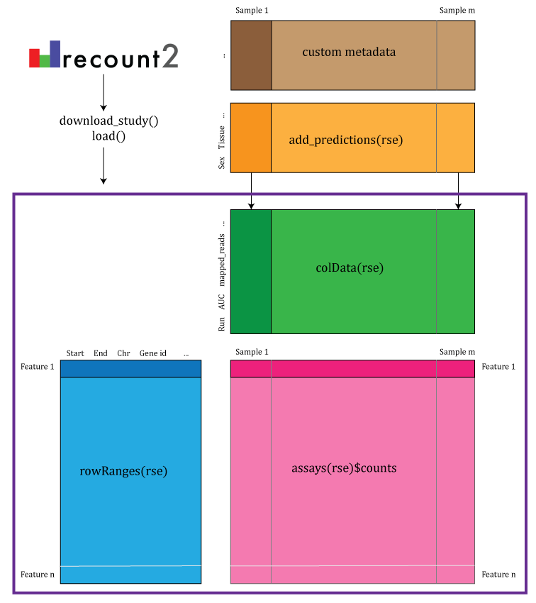
recount2 and recount3 provide coverage count matrices in
RangedSummarizedExperiment (rse) objects. Once the rse object has been
downloaded and loaded into R (using recount3::create_rse()
or recount2::download_study()), the feature information is
accessed with rowRanges(rse) (blue box), the counts with
assays(rse) (pink box) and the sample metadata with
colData(rse) (green box). The sample metadata stored in
colData(rse) can be expanded with custom code (brown box)
matching by a unique sample identifier such as the SRA Run ID. The rse
object is inside the purple box and matching data is highlighted in each
box. DOI: < https://doi.org/10.12688/f1000research.12223.1>.
recount3 enables accessing data from multiple reference organisms from public projects. To identify these projects, the key terms we use are:
- project: the project ID, which is typically the same ID that is used externally to identify that project in databases like the Sequence Read Archive 1
-
project_home: the location for where the project is
located at in the main
recount3data host: IDIES SciServer. We have two types of project homes:-
data_source: this identifies where the raw data was
downloaded from for creating
recount3. -
collection: this identifies a human-curated set of
projects or samples. The main difference compared to a
data_source is that a collection has
collection-specific metadata. For example, someone might have created a
table of information about samples in several projects by reading the
papers describing these studies as in
recount-brain(Razmara, Ellis, Sokolowski, Davis et al., 2019).
-
data_source: this identifies where the raw data was
downloaded from for creating
- organism: the reference organism (species) for the RNA-seq data, which is either human (hg38) or mouse (mm10).
Many of the recount3
raw files include three columns that are used to identify each
sample and that allow merging the data across these files. Those
are:
-
rail_id: an internal ID used by the
recountteam. The name stems fromRail-RNAwhich was the aligner used for generated the data inrecount2(Collado-Torres, Nellore, Kammers, Ellis et al., 2017). -
external_id: the external ID for the samle, such as
the Sequence Read Archive
runID. - study: the project ID.
Find a study
In order to access data from recount3, the first step is to identify a project that you are interested in working with. Most of the project IDs are the ones you can find on the Sequence Read Archive (SRA). For example, SRP009615 which we use in the examples in this vignette.The exceptions are the Genotype-Expression and The Cancer Genome Atlas human studies, commonly known as GTEx and TCGA. Both GTEx and TCGA are available in recount3 by tissue.
Through available_projects()
While you can use external websites to find a study of interest, you
can also use available_projects() to list the projects that
are available in recount3
as shown below. This will return a data.frame() object that
lists the unique project IDs.
human_projects <- available_projects()
#> 2026-04-01 03:50:56.415641 caching file sra.recount_project.MD.gz.
#> 2026-04-01 03:50:56.707845 caching file gtex.recount_project.MD.gz.
#> 2026-04-01 03:50:56.983392 caching file tcga.recount_project.MD.gz.
dim(human_projects)
#> [1] 8742    6
head(human_projects)
#>     project organism file_source     project_home project_type n_samples
#> 1 SRP107565    human         sra data_sources/sra data_sources       216
#> 2 SRP149665    human         sra data_sources/sra data_sources         4
#> 3 SRP017465    human         sra data_sources/sra data_sources        23
#> 4 SRP119165    human         sra data_sources/sra data_sources         6
#> 5 SRP133965    human         sra data_sources/sra data_sources        12
#> 6 SRP096765    human         sra data_sources/sra data_sources         7

## Select a study of interest
project_info <- subset(
    human_projects,
    project == "SRP009615" & project_type == "data_sources"
)
project_info
#>        project organism file_source     project_home project_type n_samples
#> 1838 SRP009615    human         sra data_sources/sra data_sources        12
Let’s say that you are interested in the GTEx projects, you could
then filter by file_source. We’ll focus only on those
entries that from a data source, and not from a collection for now.
subset(human_projects, file_source == "gtex" & project_type == "data_sources")
#>              project organism file_source      project_home project_type
#> 8678  ADIPOSE_TISSUE    human        gtex data_sources/gtex data_sources
#> 8679          MUSCLE    human        gtex data_sources/gtex data_sources
#> 8680    BLOOD_VESSEL    human        gtex data_sources/gtex data_sources
#> 8681           HEART    human        gtex data_sources/gtex data_sources
#> 8682           OVARY    human        gtex data_sources/gtex data_sources
#> 8683          UTERUS    human        gtex data_sources/gtex data_sources
#> 8684          VAGINA    human        gtex data_sources/gtex data_sources
#> 8685          BREAST    human        gtex data_sources/gtex data_sources
#> 8686            SKIN    human        gtex data_sources/gtex data_sources
#> 8687  SALIVARY_GLAND    human        gtex data_sources/gtex data_sources
#> 8688           BRAIN    human        gtex data_sources/gtex data_sources
#> 8689   ADRENAL_GLAND    human        gtex data_sources/gtex data_sources
#> 8690         THYROID    human        gtex data_sources/gtex data_sources
#> 8691            LUNG    human        gtex data_sources/gtex data_sources
#> 8692          SPLEEN    human        gtex data_sources/gtex data_sources
#> 8693        PANCREAS    human        gtex data_sources/gtex data_sources
#> 8694       ESOPHAGUS    human        gtex data_sources/gtex data_sources
#> 8695         STOMACH    human        gtex data_sources/gtex data_sources
#> 8696           COLON    human        gtex data_sources/gtex data_sources
#> 8697 SMALL_INTESTINE    human        gtex data_sources/gtex data_sources
#> 8698        PROSTATE    human        gtex data_sources/gtex data_sources
#> 8699          TESTIS    human        gtex data_sources/gtex data_sources
#> 8700           NERVE    human        gtex data_sources/gtex data_sources
#> 8701       PITUITARY    human        gtex data_sources/gtex data_sources
#> 8702           BLOOD    human        gtex data_sources/gtex data_sources
#> 8703           LIVER    human        gtex data_sources/gtex data_sources
#> 8704          KIDNEY    human        gtex data_sources/gtex data_sources
#> 8705    CERVIX_UTERI    human        gtex data_sources/gtex data_sources
#> 8706  FALLOPIAN_TUBE    human        gtex data_sources/gtex data_sources
#> 8707         BLADDER    human        gtex data_sources/gtex data_sources
#> 8708        STUDY_NA    human        gtex data_sources/gtex data_sources
#> 8709     BONE_MARROW    human        gtex data_sources/gtex data_sources
#>      n_samples
#> 8678      1293
#> 8679       881
#> 8680      1398
#> 8681       942
#> 8682       195
#> 8683       159
#> 8684       173
#> 8685       482
#> 8686      1940
#> 8687       178
#> 8688      2931
#> 8689       274
#> 8690       706
#> 8691       655
#> 8692       255
#> 8693       360
#> 8694      1577
#> 8695       384
#> 8696       822
#> 8697       193
#> 8698       263
#> 8699       410
#> 8700       659
#> 8701       301
#> 8702      1048
#> 8703       251
#> 8704        98
#> 8705        19
#> 8706         9
#> 8707        21
#> 8708       133
#> 8709       204
Note that one of the projects for GTEx is STUDY_NA,
that’s because in recount3
we processed all GTEx samples, including some that had no tissue
assigned and were not used by the GTEx consortium.
Ultimately, we need three pieces of information in order to download a specific dataset from recount3. Those are:
- project: the project ID,
- organism: either human or mouse,
- project_home: where the data lives which varies between data sources and collections.
project_info[, c("project", "organism", "project_home")]
#>        project organism     project_home
#> 1838 SRP009615    human data_sources/sra
Available annotations
Now that we have identified our project of interest, the next step is
to choose an annotation that we want to work with. The annotation files
available depend on the organism. To facilitate finding the specific
names we use in recount3,
we have provided the function annotation_options().
annotation_options("human")
#> [1] "gencode_v26" "gencode_v29" "fantom6_cat" "refseq"      "ercc"
#> [6] "sirv"
annotation_options("mouse")
#> [1] "gencode_v23"
The main sources are:
- GENCODE project
- RefSeq: NCBI Reference Sequence Database
- FANTOM6_CAT which was first used with
recount2(Imada, Sanchez, Collado-Torres, Wilks et al., 2020) - ERCC: External RNA Controls Consortium 2, commercially available from ThermoFisher Scientific
- SIRV 3, commercially available from Lexogen
In recount3
we have provided multiple annotations, which is different from recount
(recount2 R/Bioconductor package) where all files were
computed using GENCODE version 25. However, in both, you might be
interested in quantifying your annotation of interest, as described
further below in the BigWig files section.
Build a RSE
Once you have chosen an annotation and a project, you can now build a
RangedSummarizedExperiment object
(Huber, Carey, Gentleman,
Anders et al., 2015;
Morgan,
Obenchain, Hester, and Pagès, 2019). To do so, we recommend using
the create_rse() function as shown below for GENCODE v26
(the default annotation for human files). create_rse()
internally uses several other recount3
functions for locating the necessary raw files, downloading them,
reading them, and building the RangedSummarizedExperiment
(RSE) object. create_rse() shows several status message
updates that you can silence with
suppressMessages(create_rse()) if you want to.
## Create a RSE object at the gene level
rse_gene_SRP009615 <- create_rse(project_info)
#> 2026-04-01 03:50:59.801043 downloading and reading the metadata.
#> 2026-04-01 03:51:00.048516 caching file sra.sra.SRP009615.MD.gz.
#> 2026-04-01 03:51:00.281051 caching file sra.recount_project.SRP009615.MD.gz.
#> 2026-04-01 03:51:00.578873 caching file sra.recount_qc.SRP009615.MD.gz.
#> 2026-04-01 03:51:00.850839 caching file sra.recount_seq_qc.SRP009615.MD.gz.
#> 2026-04-01 03:51:01.098705 caching file sra.recount_pred.SRP009615.MD.gz.
#> 2026-04-01 03:51:01.160063 downloading and reading the feature information.
#> 2026-04-01 03:51:01.404486 caching file human.gene_sums.G026.gtf.gz.
#> 2026-04-01 03:51:01.852306 downloading and reading the counts: 12 samples across 63856 features.
#> 2026-04-01 03:51:02.064846 caching file sra.gene_sums.SRP009615.G026.gz.
#> 2026-04-01 03:51:02.190225 constructing the RangedSummarizedExperiment (rse) object.

## Explore the resulting RSE gene object
rse_gene_SRP009615
#> class: RangedSummarizedExperiment
#> dim: 63856 12
#> metadata(8): time_created recount3_version ... annotation recount3_url
#> assays(1): raw_counts
#> rownames(63856): ENSG00000278704.1 ENSG00000277400.1 ...
#>   ENSG00000182484.15_PAR_Y ENSG00000227159.8_PAR_Y
#> rowData names(10): source type ... havana_gene tag
#> colnames(12): SRR387777 SRR387778 ... SRR389077 SRR389078
#> colData names(175): rail_id external_id ...
#>   recount_pred.curated.cell_line BigWigURL
Explore the RSE
Because the RSE object is created at run-time in recount3,
unlike the static files provided by recount
for recount2, create_rse() stores information
about how this RSE object was made under metadata(). This
information is useful in case you share the RSE object and someone else
wants to be able to re-make the object with the latest data 4.
## Information about how this RSE object was made
metadata(rse_gene_SRP009615)
#> $time_created
#> [1] "2026-04-01 03:51:02 UTC"
#>
#> $recount3_version
#>           package ondiskversion loadedversion                        path
#> recount3 recount3        1.21.1        1.21.1 /__w/_temp/Library/recount3
#>                           loadedpath attached is_base       date       source
#> recount3 /__w/_temp/Library/recount3     TRUE   FALSE 2026-04-01 Bioconductor
#>          md5ok            library
#> recount3    NA /__w/_temp/Library
#>
#> $project
#> [1] "SRP009615"
#>
#> $project_home
#> [1] "data_sources/sra"
#>
#> $type
#> [1] "gene"
#>
#> $organism
#> [1] "human"
#>
#> $annotation
#> [1] "gencode_v26"
#>
#> $recount3_url
#> [1] "http://duffel.rail.bio/recount3"
The SRP009615 study was composed of 12 samples, for which we have
63,856 genes in GENCODE v26. The annotation-specific information is
available through rowRanges() as shown below with the
gene_id column used to identify genes in each of the
annotations 5.
## Number of genes by number of samples
dim(rse_gene_SRP009615)
#> [1] 63856    12

## Information about the genes
rowRanges(rse_gene_SRP009615)
#> GRanges object with 63856 ranges and 10 metadata columns:
#>                              seqnames            ranges strand |   source
#>                                 <Rle>         <IRanges>  <Rle> | <factor>
#>          ENSG00000278704.1 GL000009.2       56140-58376      - |  ENSEMBL
#>          ENSG00000277400.1 GL000194.1      53590-115018      - |  ENSEMBL
#>          ENSG00000274847.1 GL000194.1      53594-115055      - |  ENSEMBL
#>          ENSG00000277428.1 GL000195.1       37434-37534      - |  ENSEMBL
#>          ENSG00000276256.1 GL000195.1       42939-49164      - |  ENSEMBL
#>                        ...        ...               ...    ... .      ...
#>   ENSG00000124334.17_PAR_Y       chrY 57184101-57197337      + |   HAVANA
#>   ENSG00000185203.12_PAR_Y       chrY 57201143-57203357      - |   HAVANA
#>    ENSG00000270726.6_PAR_Y       chrY 57190738-57208756      + |   HAVANA
#>   ENSG00000182484.15_PAR_Y       chrY 57207346-57212230      + |   HAVANA
#>    ENSG00000227159.8_PAR_Y       chrY 57212184-57214397      - |   HAVANA
#>                                type bp_length     phase                gene_id
#>                            <factor> <numeric> <integer>            <character>
#>          ENSG00000278704.1     gene      2237      <NA>      ENSG00000278704.1
#>          ENSG00000277400.1     gene      2179      <NA>      ENSG00000277400.1
#>          ENSG00000274847.1     gene      1599      <NA>      ENSG00000274847.1
#>          ENSG00000277428.1     gene       101      <NA>      ENSG00000277428.1
#>          ENSG00000276256.1     gene      2195      <NA>      ENSG00000276256.1
#>                        ...      ...       ...       ...                    ...
#>   ENSG00000124334.17_PAR_Y     gene      2504      <NA> ENSG00000124334.17_P..
#>   ENSG00000185203.12_PAR_Y     gene      1054      <NA> ENSG00000185203.12_P..
#>    ENSG00000270726.6_PAR_Y     gene       773      <NA> ENSG00000270726.6_PA..
#>   ENSG00000182484.15_PAR_Y     gene      4618      <NA> ENSG00000182484.15_P..
#>    ENSG00000227159.8_PAR_Y     gene      1306      <NA> ENSG00000227159.8_PA..
#>                                         gene_type   gene_name       level
#>                                       <character> <character> <character>
#>          ENSG00000278704.1         protein_coding  BX004987.1           3
#>          ENSG00000277400.1         protein_coding  AC145212.2           3
#>          ENSG00000274847.1         protein_coding  AC145212.1           3
#>          ENSG00000277428.1               misc_RNA       Y_RNA           3
#>          ENSG00000276256.1         protein_coding  AC011043.1           3
#>                        ...                    ...         ...         ...
#>   ENSG00000124334.17_PAR_Y         protein_coding        IL9R           2
#>   ENSG00000185203.12_PAR_Y              antisense      WASIR1           2
#>    ENSG00000270726.6_PAR_Y   processed_transcript AJ271736.10           2
#>   ENSG00000182484.15_PAR_Y transcribed_unproces..      WASH6P           2
#>    ENSG00000227159.8_PAR_Y unprocessed_pseudogene    DDX11L16           2
#>                                     havana_gene         tag
#>                                     <character> <character>
#>          ENSG00000278704.1                 <NA>        <NA>
#>          ENSG00000277400.1                 <NA>        <NA>
#>          ENSG00000274847.1                 <NA>        <NA>
#>          ENSG00000277428.1                 <NA>        <NA>
#>          ENSG00000276256.1                 <NA>        <NA>
#>                        ...                  ...         ...
#>   ENSG00000124334.17_PAR_Y OTTHUMG00000022720.1         PAR
#>   ENSG00000185203.12_PAR_Y OTTHUMG00000022676.3         PAR
#>    ENSG00000270726.6_PAR_Y OTTHUMG00000184987.2         PAR
#>   ENSG00000182484.15_PAR_Y OTTHUMG00000022677.5         PAR
#>    ENSG00000227159.8_PAR_Y OTTHUMG00000022678.1         PAR
#>   -------
#>   seqinfo: 374 sequences from an unspecified genome; no seqlengths
Sample metadata
The sample metadata provided in recount3
is much more extensive than the one in recount
for the recount2 project because it’s includes for quality
control metrics, predictions, and information used
internally by recount3
functions such as create_rse(). All individual metadata
tables include the columns rail_id,
external_id and study which are used
for merging the different tables. Finally, **BigWigUrl* provides the URL
for the BigWig file for the given sample.
## Sample metadata
recount3_cols <- colnames(colData(rse_gene_SRP009615))

## How many are there?
length(recount3_cols)
#> [1] 175

## View the first few ones
head(recount3_cols)
#> [1] "rail_id"            "external_id"        "study"
#> [4] "sra.sample_acc.x"   "sra.experiment_acc" "sra.submission_acc"

## Group them by source
recount3_cols_groups <- table(gsub("\\..*", "", recount3_cols))

## Common sources and number of columns per source
recount3_cols_groups[recount3_cols_groups > 1]
#>
#>    recount_pred recount_project      recount_qc  recount_seq_qc             sra
#>               7               5             109              12              38

## Unique columns
recount3_cols_groups[recount3_cols_groups == 1]
#>
#>   BigWigURL external_id     rail_id       study
#>           1           1           1           1
## Explore them all
recount3_cols
For studies from SRA, we can further extract the SRA attributes using
expand_sra_attributes() as shown below.
rse_gene_SRP009615_expanded <-
    expand_sra_attributes(rse_gene_SRP009615)
colData(rse_gene_SRP009615_expanded)[, ncol(colData(rse_gene_SRP009615)):ncol(colData(rse_gene_SRP009615_expanded))]
#> DataFrame with 12 rows and 5 columns
#>                        BigWigURL sra_attribute.cells
#>                      <character>         <character>
#> SRR387777 http://duffel.rail.b..                K562
#> SRR387778 http://duffel.rail.b..                K562
#> SRR387779 http://duffel.rail.b..                K562
#> SRR387780 http://duffel.rail.b..                K562
#> SRR389079 http://duffel.rail.b..                K562
#> ...                          ...                 ...
#> SRR389082 http://duffel.rail.b..                K562
#> SRR389083 http://duffel.rail.b..                K562
#> SRR389084 http://duffel.rail.b..                K562
#> SRR389077 http://duffel.rail.b..                K562
#> SRR389078 http://duffel.rail.b..                K562
#>           sra_attribute.shRNA_expression sra_attribute.source_name
#>                              <character>               <character>
#> SRR387777                             no                    SL2933
#> SRR387778             yes, targeting SRF                    SL2934
#> SRR387779                             no                    SL5265
#> SRR387780              yes targeting SRF                    SL3141
#> SRR389079            no shRNA expression                    SL6485
#> ...                                  ...                       ...
#> SRR389082         expressing shRNA tar..                    SL2592
#> SRR389083            no shRNA expression                    SL4337
#> SRR389084         expressing shRNA tar..                    SL4326
#> SRR389077            no shRNA expression                    SL1584
#> SRR389078         expressing shRNA tar..                    SL1583
#>           sra_attribute.treatment
#>                       <character>
#> SRR387777               Puromycin
#> SRR387778  Puromycin, doxycycline
#> SRR387779               Puromycin
#> SRR387780  Puromycin, doxycycline
#> SRR389079               Puromycin
#> ...                           ...
#> SRR389082  Puromycin, doxycycline
#> SRR389083               Puromycin
#> SRR389084  Puromycin, doxycycline
#> SRR389077               Puromycin
#> SRR389078  Puromycin, doxycycline
Counts
The counts in recount3 are raw base-pair coverage counts, similar to those in recount. To further understand them, check the recountWorkflow DOI 10.12688/f1000research.12223.1. To highlight that these are raw base-pair coverage counts, they are stored in the “raw_counts” assay
assayNames(rse_gene_SRP009615)
#> [1] "raw_counts"
Using transform_counts() you can scale the counts and
assign them to the “counts” assays slot to use them in downstream
packages such as DESeq2 and
limma.
## Once you have your RSE object, you can transform the raw coverage
## base-pair coverage counts using transform_counts().
## For RPKM, TPM or read outputs, check the details in transform_counts().
assay(rse_gene_SRP009615, "counts") <- transform_counts(rse_gene_SRP009615)
Just like with recount
for recount2, you can transform the raw base-pair coverage
counts
(Collado-Torres,
Nellore, and Jaffe, 2017) to read counts with
compute_read_counts(), RPKM with
recount::getRPKM() or TPM values with
recount::getTPM(). Check transform_counts()
from recount3
for more details.
Exon
recount3
provides an interface to raw
files that go beyond gene counts, as well as other features you
might be interested in. For instance, you might want to study expression
at the exon expression level instead of
gene. To do so, use the type argument in
create_rse() as shown below.
## Create a RSE object at the exon level
rse_exon_SRP009615 <- create_rse(
    proj_info,
    type = "exon"
)
#> 2026-04-01 03:51:02.856476 downloading and reading the metadata.
#> 2026-04-01 03:51:03.129772 caching file sra.sra.SRP009615.MD.gz.
#> 2026-04-01 03:51:03.390558 caching file sra.recount_project.SRP009615.MD.gz.
#> 2026-04-01 03:51:03.661447 caching file sra.recount_qc.SRP009615.MD.gz.
#> 2026-04-01 03:51:03.916142 caching file sra.recount_seq_qc.SRP009615.MD.gz.
#> 2026-04-01 03:51:04.162602 caching file sra.recount_pred.SRP009615.MD.gz.
#> 2026-04-01 03:51:04.222366 downloading and reading the feature information.
#> 2026-04-01 03:51:04.416472 caching file human.exon_sums.G026.gtf.gz.
#> 2026-04-01 03:51:21.568687 downloading and reading the counts: 12 samples across 1299686 features.
#> 2026-04-01 03:51:21.905806 caching file sra.exon_sums.SRP009615.G026.gz.
#> 2026-04-01 03:51:23.959153 constructing the RangedSummarizedExperiment (rse) object.

## Explore the resulting RSE exon object
rse_exon_SRP009615
#> class: RangedSummarizedExperiment
#> dim: 1299686 12
#> metadata(8): time_created recount3_version ... annotation recount3_url
#> assays(1): raw_counts
#> rownames(1299686): GL000009.2|56140|58376|- GL000194.1|53594|54832|-
#>   ... chrY|57213880|57213964|- chrY|57214350|57214397|-
#> rowData names(21): source type ... ont ccdsid
#> colnames(12): SRR387777 SRR387778 ... SRR389077 SRR389078
#> colData names(175): rail_id external_id ...
#>   recount_pred.curated.cell_line BigWigURL

## Explore the object
dim(rse_exon_SRP009615)
#> [1] 1299686      12
Each exon is shown in this output, so, you might have to filter the
exons of interest. Unlike in recount2, these are actual
exons and not disjoint exons 6.
## Exon annotation information
rowRanges(rse_exon_SRP009615)
#> GRanges object with 1299686 ranges and 21 metadata columns:
#>                                seqnames            ranges strand |   source
#>                                   <Rle>         <IRanges>  <Rle> | <factor>
#>     GL000009.2|56140|58376|- GL000009.2       56140-58376      - |  ENSEMBL
#>     GL000194.1|53594|54832|- GL000194.1       53594-54832      - |  ENSEMBL
#>     GL000194.1|55446|55676|- GL000194.1       55446-55676      - |  ENSEMBL
#>     GL000194.1|53590|55676|- GL000194.1       53590-55676      - |  ENSEMBL
#>   GL000194.1|112792|112850|- GL000194.1     112792-112850      - |  ENSEMBL
#>                          ...        ...               ...    ... .      ...
#>     chrY|57212184|57213125|-       chrY 57212184-57213125      - |   HAVANA
#>     chrY|57213204|57213357|-       chrY 57213204-57213357      - |   HAVANA
#>     chrY|57213526|57213602|-       chrY 57213526-57213602      - |   HAVANA
#>     chrY|57213880|57213964|-       chrY 57213880-57213964      - |   HAVANA
#>     chrY|57214350|57214397|-       chrY 57214350-57214397      - |   HAVANA
#>                                  type bp_length     phase
#>                              <factor> <numeric> <integer>
#>     GL000009.2|56140|58376|-     exon      2237      <NA>
#>     GL000194.1|53594|54832|-     exon      1239      <NA>
#>     GL000194.1|55446|55676|-     exon       231      <NA>
#>     GL000194.1|53590|55676|-     exon      2087      <NA>
#>   GL000194.1|112792|112850|-     exon        59      <NA>
#>                          ...      ...       ...       ...
#>     chrY|57212184|57213125|-     exon       942      <NA>
#>     chrY|57213204|57213357|-     exon       154      <NA>
#>     chrY|57213526|57213602|-     exon        77      <NA>
#>     chrY|57213880|57213964|-     exon        85      <NA>
#>     chrY|57214350|57214397|-     exon        48      <NA>
#>                                             gene_id          transcript_id
#>                                         <character>            <character>
#>     GL000009.2|56140|58376|-      ENSG00000278704.1      ENST00000618686.1
#>     GL000194.1|53594|54832|-      ENSG00000274847.1      ENST00000400754.4
#>     GL000194.1|55446|55676|-      ENSG00000274847.1      ENST00000400754.4
#>     GL000194.1|53590|55676|-      ENSG00000277400.1      ENST00000613230.1
#>   GL000194.1|112792|112850|-      ENSG00000274847.1      ENST00000400754.4
#>                          ...                    ...                    ...
#>     chrY|57212184|57213125|- ENSG00000227159.8_PA.. ENST00000507418.6_PA..
#>     chrY|57213204|57213357|- ENSG00000227159.8_PA.. ENST00000507418.6_PA..
#>     chrY|57213526|57213602|- ENSG00000227159.8_PA.. ENST00000507418.6_PA..
#>     chrY|57213880|57213964|- ENSG00000227159.8_PA.. ENST00000507418.6_PA..
#>     chrY|57214350|57214397|- ENSG00000227159.8_PA.. ENST00000507418.6_PA..
#>                                           gene_type   gene_name
#>                                         <character> <character>
#>     GL000009.2|56140|58376|-         protein_coding  BX004987.1
#>     GL000194.1|53594|54832|-         protein_coding  AC145212.1
#>     GL000194.1|55446|55676|-         protein_coding  AC145212.1
#>     GL000194.1|53590|55676|-         protein_coding  AC145212.2
#>   GL000194.1|112792|112850|-         protein_coding  AC145212.1
#>                          ...                    ...         ...
#>     chrY|57212184|57213125|- unprocessed_pseudogene    DDX11L16
#>     chrY|57213204|57213357|- unprocessed_pseudogene    DDX11L16
#>     chrY|57213526|57213602|- unprocessed_pseudogene    DDX11L16
#>     chrY|57213880|57213964|- unprocessed_pseudogene    DDX11L16
#>     chrY|57214350|57214397|- unprocessed_pseudogene    DDX11L16
#>                                     transcript_type transcript_name exon_number
#>                                         <character>     <character> <character>
#>     GL000009.2|56140|58376|-         protein_coding  BX004987.1-201           1
#>     GL000194.1|53594|54832|-         protein_coding  AC145212.1-201           4
#>     GL000194.1|55446|55676|-         protein_coding  AC145212.1-201           3
#>     GL000194.1|53590|55676|-         protein_coding  AC145212.2-201           3
#>   GL000194.1|112792|112850|-         protein_coding  AC145212.1-201           2
#>                          ...                    ...             ...         ...
#>     chrY|57212184|57213125|- unprocessed_pseudogene    DDX11L16-001           5
#>     chrY|57213204|57213357|- unprocessed_pseudogene    DDX11L16-001           4
#>     chrY|57213526|57213602|- unprocessed_pseudogene    DDX11L16-001           3
#>     chrY|57213880|57213964|- unprocessed_pseudogene    DDX11L16-001           2
#>     chrY|57214350|57214397|- unprocessed_pseudogene    DDX11L16-001           1
#>                                        exon_id       level        protein_id
#>                                    <character> <character>       <character>
#>     GL000009.2|56140|58376|- ENSE00003753029.1           3 ENSP00000484918.1
#>     GL000194.1|53594|54832|- ENSE00002218789.2           3 ENSP00000478910.1
#>     GL000194.1|55446|55676|- ENSE00003714436.1           3 ENSP00000478910.1
#>     GL000194.1|53590|55676|- ENSE00003723764.1           3 ENSP00000483280.1
#>   GL000194.1|112792|112850|- ENSE00003713687.1           3 ENSP00000478910.1
#>                          ...               ...         ...               ...
#>     chrY|57212184|57213125|- ENSE00002023900.1           2              <NA>
#>     chrY|57213204|57213357|- ENSE00002036959.1           2              <NA>
#>     chrY|57213526|57213602|- ENSE00002021169.1           2              <NA>
#>     chrY|57213880|57213964|- ENSE00002046926.1           2              <NA>
#>     chrY|57214350|57214397|- ENSE00002072208.1           2              <NA>
#>                              transcript_support_level         tag
#>                                           <character> <character>
#>     GL000009.2|56140|58376|-                       NA       basic
#>     GL000194.1|53594|54832|-                        1       basic
#>     GL000194.1|55446|55676|-                        1       basic
#>     GL000194.1|53590|55676|-                        1       basic
#>   GL000194.1|112792|112850|-                        1       basic
#>                          ...                      ...         ...
#>     chrY|57212184|57213125|-                       NA         PAR
#>     chrY|57213204|57213357|-                       NA         PAR
#>     chrY|57213526|57213602|-                       NA         PAR
#>     chrY|57213880|57213964|-                       NA         PAR
#>     chrY|57214350|57214397|-                       NA         PAR
#>                                     recount_exon_id          havana_gene
#>                                         <character>          <character>
#>     GL000009.2|56140|58376|- GL000009.2|56140|583..                 <NA>
#>     GL000194.1|53594|54832|- GL000194.1|53594|548..                 <NA>
#>     GL000194.1|55446|55676|- GL000194.1|55446|556..                 <NA>
#>     GL000194.1|53590|55676|- GL000194.1|53590|556..                 <NA>
#>   GL000194.1|112792|112850|- GL000194.1|112792|11..                 <NA>
#>                          ...                    ...                  ...
#>     chrY|57212184|57213125|- chrY|57212184|572131.. OTTHUMG00000022678.1
#>     chrY|57213204|57213357|- chrY|57213204|572133.. OTTHUMG00000022678.1
#>     chrY|57213526|57213602|- chrY|57213526|572136.. OTTHUMG00000022678.1
#>     chrY|57213880|57213964|- chrY|57213880|572139.. OTTHUMG00000022678.1
#>     chrY|57214350|57214397|- chrY|57214350|572143.. OTTHUMG00000022678.1
#>                                 havana_transcript         ont      ccdsid
#>                                       <character> <character> <character>
#>     GL000009.2|56140|58376|-                 <NA>        <NA>        <NA>
#>     GL000194.1|53594|54832|-                 <NA>        <NA>        <NA>
#>     GL000194.1|55446|55676|-                 <NA>        <NA>        <NA>
#>     GL000194.1|53590|55676|-                 <NA>        <NA>        <NA>
#>   GL000194.1|112792|112850|-                 <NA>        <NA>        <NA>
#>                          ...                  ...         ...         ...
#>     chrY|57212184|57213125|- OTTHUMT00000058841.1 PGO:0000005        <NA>
#>     chrY|57213204|57213357|- OTTHUMT00000058841.1 PGO:0000005        <NA>
#>     chrY|57213526|57213602|- OTTHUMT00000058841.1 PGO:0000005        <NA>
#>     chrY|57213880|57213964|- OTTHUMT00000058841.1 PGO:0000005        <NA>
#>     chrY|57214350|57214397|- OTTHUMT00000058841.1 PGO:0000005        <NA>
#>   -------
#>   seqinfo: 374 sequences from an unspecified genome; no seqlengths

## Exon ids are repeated because a given exon can be part of
## more than one transcript
length(unique(rowRanges(rse_exon_SRP009615)$exon_id))
#> [1] 742049
Because there are many more exons than genes, this type of analysis
uses more computational resources. Thus, for some large projects you
might need to use a high performance computing environment. To help you
proceed with caution, create_rse() shows how many features
and samples it’s trying to access. So if you get an out of memory error,
you’ll know why that happened.
Exon-exon junctions
In recount3 we have also provided the option to create RSE files for exon-exon junctions. Unlike the gene/exon RSE files, only the junctions present in a given project are included in the files, so you’ll have to be more careful when merging exon-exon junction RSE files. Furthermore, these are actual read counts and not raw base-pair counts. Given the sparsity of the data, the counts are provided using a sparse matrix object from Matrix. Thus exon-exon junction files can be less memory demanding than the exon RSE files.
## Create a RSE object at the exon-exon junction level
rse_jxn_SRP009615 <- create_rse(
    proj_info,
    type = "jxn"
)
#> 2026-04-01 03:51:28.161633 downloading and reading the metadata.
#> 2026-04-01 03:51:28.463445 caching file sra.sra.SRP009615.MD.gz.
#> 2026-04-01 03:51:28.696404 caching file sra.recount_project.SRP009615.MD.gz.
#> 2026-04-01 03:51:28.996208 caching file sra.recount_qc.SRP009615.MD.gz.
#> 2026-04-01 03:51:29.257767 caching file sra.recount_seq_qc.SRP009615.MD.gz.
#> 2026-04-01 03:51:29.599066 caching file sra.recount_pred.SRP009615.MD.gz.
#> 2026-04-01 03:51:29.655667 downloading and reading the feature information.
#> 2026-04-01 03:51:29.875682 caching file sra.junctions.SRP009615.ALL.RR.gz.
#> 2026-04-01 03:51:31.162956 downloading and reading the counts: 12 samples across 281448 features.
#> 2026-04-01 03:51:31.393538 caching file sra.junctions.SRP009615.ALL.MM.gz.
#> 2026-04-01 03:51:31.812642 matching exon-exon junction counts with the metadata.
#> 2026-04-01 03:51:32.010327 caching file sra.junctions.SRP009615.ALL.ID.gz.
#> 2026-04-01 03:51:32.085446 constructing the RangedSummarizedExperiment (rse) object.

## Explore the resulting RSE exon-exon junctions object
rse_jxn_SRP009615
#> class: RangedSummarizedExperiment
#> dim: 281448 12
#> metadata(9): time_created recount3_version ... jxn_format recount3_url
#> assays(1): counts
#> rownames(281448): chr1:11845-12009:+ chr1:12698-13220:+ ...
#>   chrY:56848810-56851543:- chrY:56850515-56850921:+
#> rowData names(6): length annotated ... left_annotated right_annotated
#> colnames(12): SRR387777 SRR387778 ... SRR389077 SRR389078
#> colData names(175): rail_id external_id ...
#>   recount_pred.curated.cell_line BigWigURL
dim(rse_jxn_SRP009615)
#> [1] 281448     12

## Exon-exon junction information
rowRanges(rse_jxn_SRP009615)
#> GRanges object with 281448 ranges and 6 metadata columns:
#>                            seqnames            ranges strand |    length
#>                               <Rle>         <IRanges>  <Rle> | <integer>
#>         chr1:11845-12009:+     chr1       11845-12009      + |       165
#>         chr1:12698-13220:+     chr1       12698-13220      + |       523
#>        chr1:14696-185174:-     chr1      14696-185174      - |    170479
#>         chr1:14830-14969:-     chr1       14830-14969      - |       140
#>         chr1:14830-15020:-     chr1       14830-15020      - |       191
#>                        ...      ...               ...    ... .       ...
#>   chrY:56846131-56846553:+     chrY 56846131-56846553      + |       423
#>   chrY:56846268-56846553:+     chrY 56846268-56846553      + |       286
#>   chrY:56846486-56846553:+     chrY 56846486-56846553      + |        68
#>   chrY:56848810-56851543:-     chrY 56848810-56851543      - |      2734
#>   chrY:56850515-56850921:+     chrY 56850515-56850921      + |       407
#>                            annotated  left_motif right_motif
#>                            <integer> <character> <character>
#>         chr1:11845-12009:+         0          GT          AG
#>         chr1:12698-13220:+         1          GT          AG
#>        chr1:14696-185174:-         0          CT          AC
#>         chr1:14830-14969:-         1          CT          AC
#>         chr1:14830-15020:-         0          CT          AC
#>                        ...       ...         ...         ...
#>   chrY:56846131-56846553:+         0          GT          AG
#>   chrY:56846268-56846553:+         0          GT          AG
#>   chrY:56846486-56846553:+         0          GT          AG
#>   chrY:56848810-56851543:-         0          CT          AC
#>   chrY:56850515-56850921:+         0          GT          AG
#>                                    left_annotated        right_annotated
#>                                       <character>            <character>
#>         chr1:11845-12009:+                      0              aC19,sG19
#>         chr1:12698-13220:+ aC19,gC19,gC24,gC25,.. aC19,cH38,gC19,gC24,..
#>        chr1:14696-185174:-                      0                      0
#>         chr1:14830-14969:- aC19,cH38,gC19,kG19,.. aC19,cH38,gC19,kG19,..
#>         chr1:14830-15020:- aC19,cH38,gC19,kG19,..                      0
#>                        ...                    ...                    ...
#>   chrY:56846131-56846553:+                      0                      0
#>   chrY:56846268-56846553:+                      0                      0
#>   chrY:56846486-56846553:+                      0                      0
#>   chrY:56848810-56851543:-                      0                      0
#>   chrY:56850515-56850921:+                      0                      0
#>   -------
#>   seqinfo: 97 sequences from an unspecified genome; no seqlengths

## Memory used
lobstr::obj_size(rse_jxn_SRP009615)
#> 60.30 MB
BigWig files
Internally we used GenomicFeatures::exonicParts() when
processing all annotations in recount3
instead of GenomicRanges::disjoin() that was used in
recount2. We then re-assembled the counts for each
exon/gene to create the count files provided in recount3.
However, you might want to exclude the overlapping exonic parts from the
counts. If that’s the case or if you are interested in specific regions
of the hg38/mm10 genomes, you might want to
access the coverage BigWig files.
## BigWig file names
## The full URL is stored in BigWigUrl
basename(head(rse_gene_SRP009615$BigWigURL))
#> [1] "sra.base_sums.SRP009615_SRR387777.ALL.bw"
#> [2] "sra.base_sums.SRP009615_SRR387778.ALL.bw"
#> [3] "sra.base_sums.SRP009615_SRR387779.ALL.bw"
#> [4] "sra.base_sums.SRP009615_SRR387780.ALL.bw"
#> [5] "sra.base_sums.SRP009615_SRR389079.ALL.bw"
#> [6] "sra.base_sums.SRP009615_SRR389080.ALL.bw"
These BigWig files can be accessed using
rtracklayer::import.bw() from R, or other tools such as bwtool that
we’ve used in the past 7. Using them, you can compute a coverage
matrix for a given set of regions.
One new software we developed is megadepth
for which we have provided an R/Bioconductor package interface. megadepth
is faster at accessing BigWig files and is the software we used
internally for generating the recount3 data. megadepth
provides convenient to use functions for quantifying a set of regions,
which might be of interest for co-expression analyses where double
counting exonic parts can be problematic.
You can also use derfinder and derfinderPlot if you are interested in visualizing the base-pair coverage data for a specific region using these BigWig coverage files.
Local files
recount3 depends on BiocFileCache (Shepherd and Morgan, 2025) for organizing the raw files and caching them, such that if you use the same file more than once, you only have to download it once. BiocFileCache will automatically update the file if it detects that the file has changed in the source
If you want to inspect which files you have downloaded or even delete
them, them you’ll want to use recount3_cache_files() and
recount3_cache_rm() as illustrated below.
## List the URLs of the recount3 data that you have downloaded
recount3_cache_files()
#>  [1] "http://duffel.rail.bio/recount3/human/data_sources/sra/metadata/sra.recount_project.MD.gz"
#>  [2] "http://duffel.rail.bio/recount3/human/data_sources/gtex/metadata/gtex.recount_project.MD.gz"
#>  [3] "http://duffel.rail.bio/recount3/human/data_sources/tcga/metadata/tcga.recount_project.MD.gz"
#>  [4] "http://duffel.rail.bio/recount3/human/data_sources/sra/metadata/15/SRP009615/sra.sra.SRP009615.MD.gz"
#>  [5] "http://duffel.rail.bio/recount3/human/data_sources/sra/metadata/15/SRP009615/sra.recount_project.SRP009615.MD.gz"
#>  [6] "http://duffel.rail.bio/recount3/human/data_sources/sra/metadata/15/SRP009615/sra.recount_qc.SRP009615.MD.gz"
#>  [7] "http://duffel.rail.bio/recount3/human/data_sources/sra/metadata/15/SRP009615/sra.recount_seq_qc.SRP009615.MD.gz"
#>  [8] "http://duffel.rail.bio/recount3/human/data_sources/sra/metadata/15/SRP009615/sra.recount_pred.SRP009615.MD.gz"
#>  [9] "http://duffel.rail.bio/recount3/human/annotations/gene_sums/human.gene_sums.G026.gtf.gz"
#> [10] "http://duffel.rail.bio/recount3/human/data_sources/sra/gene_sums/15/SRP009615/sra.gene_sums.SRP009615.G026.gz"
#> [11] "http://duffel.rail.bio/recount3/human/annotations/exon_sums/human.exon_sums.G026.gtf.gz"
#> [12] "http://duffel.rail.bio/recount3/human/data_sources/sra/exon_sums/15/SRP009615/sra.exon_sums.SRP009615.G026.gz"
#> [13] "http://duffel.rail.bio/recount3/human/data_sources/sra/junctions/15/SRP009615/sra.junctions.SRP009615.ALL.RR.gz"
#> [14] "http://duffel.rail.bio/recount3/human/data_sources/sra/junctions/15/SRP009615/sra.junctions.SRP009615.ALL.MM.gz"
#> [15] "http://duffel.rail.bio/recount3/human/data_sources/sra/junctions/15/SRP009615/sra.junctions.SRP009615.ALL.ID.gz"
#> [16] "http://duffel.rail.bio/recount3/mouse/data_sources/sra/metadata/sra.recount_project.MD.gz"
#> [17] "http://duffel.rail.bio/recount3/human/data_sources/sra/metadata/99/DRP000499/sra.sra.DRP000499.MD.gz"
#> [18] "http://duffel.rail.bio/recount3/human/data_sources/sra/metadata/99/DRP000499/sra.recount_project.DRP000499.MD.gz"
#> [19] "http://duffel.rail.bio/recount3/human/data_sources/sra/metadata/99/DRP000499/sra.recount_qc.DRP000499.MD.gz"
#> [20] "http://duffel.rail.bio/recount3/human/data_sources/sra/metadata/99/DRP000499/sra.recount_seq_qc.DRP000499.MD.gz"
#> [21] "http://duffel.rail.bio/recount3/human/data_sources/sra/metadata/99/DRP000499/sra.recount_pred.DRP000499.MD.gz"
#> [22] "http://duffel.rail.bio/recount3/human/data_sources/sra/gene_sums/99/DRP000499/sra.gene_sums.DRP000499.G026.gz"
#> [23] "http://duffel.rail.bio/recount3/human/annotations/gene_sums/human.gene_sums.G029.gtf.gz"
#> [24] "http://duffel.rail.bio/recount3/human/data_sources/sra/gene_sums/15/SRP009615/sra.gene_sums.SRP009615.G029.gz"
#> [25] "http://duffel.rail.bio/recount3/human/annotations/gene_sums/human.gene_sums.F006.gtf.gz"
#> [26] "http://duffel.rail.bio/recount3/human/data_sources/sra/gene_sums/15/SRP009615/sra.gene_sums.SRP009615.F006.gz"
#> [27] "http://duffel.rail.bio/recount3/human/annotations/gene_sums/human.gene_sums.R109.gtf.gz"
#> [28] "http://duffel.rail.bio/recount3/human/data_sources/sra/gene_sums/15/SRP009615/sra.gene_sums.SRP009615.R109.gz"
#> [29] "http://duffel.rail.bio/recount3/human/annotations/gene_sums/human.gene_sums.ERCC.gtf.gz"
#> [30] "http://duffel.rail.bio/recount3/human/data_sources/sra/gene_sums/15/SRP009615/sra.gene_sums.SRP009615.ERCC.gz"
#> [31] "http://duffel.rail.bio/recount3/human/annotations/gene_sums/human.gene_sums.SIRV.gtf.gz"
#> [32] "http://duffel.rail.bio/recount3/human/data_sources/sra/gene_sums/15/SRP009615/sra.gene_sums.SRP009615.SIRV.gz"
#> [33] "http://snaptron.cs.jhu.edu/data/temp/recount3/human/collections/geuvadis_smartseq/metadata/geuvadis_smartseq.recount_project.gz"
#> [34] "http://snaptron.cs.jhu.edu/data/temp/recount3/human/data_sources/sra/metadata/66/ERP110066/sra.sra.ERP110066.MD.gz"
#> [35] "http://snaptron.cs.jhu.edu/data/temp/recount3/human/data_sources/sra/metadata/66/ERP110066/sra.recount_project.ERP110066.MD.gz"
#> [36] "http://snaptron.cs.jhu.edu/data/temp/recount3/human/data_sources/sra/metadata/66/ERP110066/sra.recount_qc.ERP110066.MD.gz"
#> [37] "http://snaptron.cs.jhu.edu/data/temp/recount3/human/data_sources/sra/metadata/66/ERP110066/sra.recount_pred.ERP110066.MD.gz"
#> [38] "http://snaptron.cs.jhu.edu/data/temp/recount3/human/collections/geuvadis_smartseq/metadata/geuvadis_smartseq.custom.gz"
#> [39] "http://snaptron.cs.jhu.edu/data/temp/recount3/human/annotations/gene_sums/human.gene_sums.G026.gtf.gz"
#> [40] "http://snaptron.cs.jhu.edu/data/temp/recount3/human/data_sources/sra/gene_sums/66/ERP110066/sra.gene_sums.ERP110066.G026.gz"
#> [41] "http://duffel.rail.bio/recount3/mouse/data_sources/sra/metadata/67/DRP002367/sra.sra.DRP002367.MD.gz"
#> [42] "http://duffel.rail.bio/recount3/mouse/data_sources/sra/metadata/67/DRP002367/sra.recount_project.DRP002367.MD.gz"
#> [43] "http://duffel.rail.bio/recount3/mouse/data_sources/sra/metadata/67/DRP002367/sra.recount_qc.DRP002367.MD.gz"
#> [44] "http://duffel.rail.bio/recount3/mouse/data_sources/sra/metadata/67/DRP002367/sra.recount_seq_qc.DRP002367.MD.gz"
#> [45] "http://duffel.rail.bio/recount3/mouse/data_sources/sra/metadata/67/DRP002367/sra.recount_pred.DRP002367.MD.gz"
#> [46] "http://duffel.rail.bio/recount3/mouse/annotations/gene_sums/mouse.gene_sums.M023.gtf.gz"
#> [47] "http://duffel.rail.bio/recount3/mouse/data_sources/sra/gene_sums/67/DRP002367/sra.gene_sums.DRP002367.M023.gz"
#> [48] "http://duffel.rail.bio/recount3/human/data_sources/sra/metadata/66/ERP110066/sra.sra.ERP110066.MD.gz"
#> [49] "http://duffel.rail.bio/recount3/human/data_sources/sra/metadata/66/ERP110066/sra.recount_project.ERP110066.MD.gz"
#> [50] "http://duffel.rail.bio/recount3/human/data_sources/sra/metadata/66/ERP110066/sra.recount_qc.ERP110066.MD.gz"
#> [51] "http://duffel.rail.bio/recount3/human/data_sources/sra/metadata/66/ERP110066/sra.recount_seq_qc.ERP110066.MD.gz"
#> [52] "http://duffel.rail.bio/recount3/human/data_sources/sra/metadata/66/ERP110066/sra.recount_pred.ERP110066.MD.gz"
#> [53] "http://duffel.rail.bio/recount3/human/data_sources/gtex/metadata/ER/BLADDER/gtex.gtex.BLADDER.MD.gz"
#> [54] "http://duffel.rail.bio/recount3/human/data_sources/gtex/metadata/ER/BLADDER/gtex.recount_project.BLADDER.MD.gz"
#> [55] "http://duffel.rail.bio/recount3/human/data_sources/gtex/metadata/ER/BLADDER/gtex.recount_qc.BLADDER.MD.gz"
#> [56] "http://duffel.rail.bio/recount3/human/data_sources/gtex/metadata/ER/BLADDER/gtex.recount_seq_qc.BLADDER.MD.gz"
#> [57] "https://idies.jhu.edu/recount3/data/human/data_sources/sra/metadata/sra.recount_project.MD.gz"
#> [58] "https://idies.jhu.edu/recount3/data/human/data_sources/gtex/metadata/gtex.recount_project.MD.gz"
#> [59] "https://idies.jhu.edu/recount3/data/human/data_sources/tcga/metadata/tcga.recount_project.MD.gz"
#> [60] "https://idies.jhu.edu/recount3/data/mouse/data_sources/sra/metadata/sra.recount_project.MD.gz"
#> [61] "https://data.idies.jhu.edu/recount3/data//human/data_sources/sra/metadata/sra.recount_project.MD.gz"
#> [62] "https://data.idies.jhu.edu/recount3/data//human/data_sources/gtex/metadata/gtex.recount_project.MD.gz"
#> [63] "https://data.idies.jhu.edu/recount3/data//human/data_sources/tcga/metadata/tcga.recount_project.MD.gz"
#> [64] "http://duffel.rail.bio/recount3/human/data_sources/sra/metadata/67/SRP103067/sra.sra.SRP103067.MD.gz"
#> [65] "http://duffel.rail.bio/recount3/human/data_sources/sra/metadata/67/SRP103067/sra.recount_project.SRP103067.MD.gz"
#> [66] "http://duffel.rail.bio/recount3/human/data_sources/sra/metadata/67/SRP103067/sra.recount_qc.SRP103067.MD.gz"
#> [67] "http://duffel.rail.bio/recount3/human/data_sources/sra/metadata/67/SRP103067/sra.recount_seq_qc.SRP103067.MD.gz"
#> [68] "http://duffel.rail.bio/recount3/human/data_sources/sra/metadata/67/SRP103067/sra.recount_pred.SRP103067.MD.gz"
## Delete the recount3 files from your cache
recount3_cache_rm()

## Check that no files are listed
recount3_cache_files()
Your own mirror
recount3
functions such as create_rse() have a
recount3_url argument that can be changed to point to a
mirror or to a path in your computing system. This argument enables
using recount3
with data stored in other locations, or even generated using the same
processing pipeline that was used for recount3
but for your own/private data.
The main documentation website documents how the raw files should be
organized in your mirror or for your own data. You can inspect the
structure of the data by checking the internals of
locate_url() and locate_url_ann(). Both
functions can be used to get the full list of URLs. In addition, for a
given mirror, available_projects() will show the local data
sources and collections. Finally, file_retrieve() won’t
cache the data if it detects that the data already exists in the local
disk.
In particular, this functionality can be useful if you want to access
the data through Registry of Open Data on
AWS or at IDIES using SciServer Compute, which
are the two official mirrors for recount3 data.
![]()
![]()
Teams involved
The ReCount family involves the following teams:
- Ben Langmead’s lab at JHU Computer Science
- Kasper Daniel Hansen’s lab at JHBSPH Biostatistics Department
- Leonardo Collado-Torres and Andrew E. Jaffe from LIBD
- Abhinav Nellore’s lab at OHSU
- Jeff Leek’s lab at JHBSPH Biostatistics Deparment
- Data hosted by the Registry of Open Data on AWS and SciServer from IDIES at JHU through a load balancer called duffel.
Project history
To clarify the relationship between the R/Bioconductor packages and
the phases of ReCount
(Frazee,
Langmead, and Leek, 2011) please check the table below:
| Year | Phase | Main references | R/Bioconductor |
|---|---|---|---|
| 2011 | ReCount |
DOI: 10.1186/1471-2105-12-449 | none |
| 2017 | recount2 |
DOI: 10.1038/nbt.3838 10.12688/f1000research.12223.1 | recount |
| 2021 | recount3 |
DOI: 10.1186/s13059-021-02533-6 | recount3 |
Other related tools
The ReCount team has worked on several software
solutions and projects that complement each other and enable you to
re-use public RNA-seq data. Another Bioconductor package that you might
be highly interested in is snapcount,
which allows you to use the Snaptron web services. In
particular, snapcount
is best for queries over a particular subset of genes or intervals
across all or most of the samples in
recount2/Snaptron.
We remind you that the main documentation website
for all the recount3-related projects is available at recount.bio.
Please check that website for more information about how this
R/Bioconductor package and other tools are related to each other.
Thank you!
P.S. An alternative version of this vignette is available that was made using pkgdown.
Reproducibility
The recount3 package (Collado-Torres, 2026) was made possible thanks to:
- R (R Core Team, 2026)
- BiocFileCache (Shepherd and Morgan, 2025)
- BiocStyle (Oleś, 2025)
- biocthis
- covr (Hester, 2025)
- data.table (Barrett, Dowle, Srinivasan, Gorecki et al., 2026)
- GenomicRanges (Lawrence, Huber, Pagès, Aboyoun et al., 2013)
- httr (Wickham, 2026)
- knitcitations (Boettiger, 2021)
- knitr (Xie, 2014)
- lobstr (Wickham, 2026)
- Matrix (Bates, Maechler, and Jagan, 2026)
- R.utils (Bengtsson, 2025)
- RefManageR (McLean, 2017)
- rmarkdown (Allaire, Xie, Dervieux, McPherson et al., 2026)
- rtracklayer (Lawrence, Gentleman, and Carey, 2009)
- S4Vectors (Pagès, Lawrence, and Aboyoun, 2025)
- sessioninfo (Wickham, Chang, Flight, Müller et al., 2025)
- SummarizedExperiment (Morgan, Obenchain, Hester, and Pagès, 2019)
- testthat (Wickham, 2011)
Code for creating the vignette
## Create the vignette
library("rmarkdown")
system.time(render("recount3-quickstart.Rmd", "BiocStyle::html_document"))

## Extract the R code
library("knitr")
knit("recount3-quickstart.Rmd", tangle = TRUE)
## Clean up
file.remove("quickstartRef.bib")
#> [1] TRUE
Date the vignette was generated.
#> [1] "2026-04-01 03:51:33 UTC"Wallclock time spent generating the vignette.
#> Time difference of 54.629 secsR session information.
#> ─ Session info ───────────────────────────────────────────────────────────────────────────────────────────────────────
#>  setting  value
#>  version  R Under development (unstable) (2026-03-28 r89738)
#>  os       Ubuntu 24.04.4 LTS
#>  system   x86_64, linux-gnu
#>  ui       X11
#>  language en
#>  collate  en_US.UTF-8
#>  ctype    en_US.UTF-8
#>  tz       UTC
#>  date     2026-04-01
#>  pandoc   3.9.0.2 @ /usr/bin/ (via rmarkdown)
#>  quarto   1.8.25 @ /usr/local/bin/quarto
#>
#> ─ Packages ───────────────────────────────────────────────────────────────────────────────────────────────────────────
#>  package              * version    date (UTC) lib source
#>  abind                  1.4-8      2024-09-12 [1] CRAN (R 4.6.0)
#>  backports              1.5.0      2024-05-23 [1] CRAN (R 4.6.0)
#>  bibtex                 0.5.2      2026-02-03 [1] CRAN (R 4.6.0)
#>  Biobase              * 2.71.0     2025-10-30 [1] Bioconductor 3.23 (R 4.6.0)
#>  BiocFileCache          3.1.0      2025-10-30 [1] Bioconductor 3.23 (R 4.6.0)
#>  BiocGenerics         * 0.57.0     2025-10-30 [1] Bioconductor 3.23 (R 4.6.0)
#>  BiocIO                 1.21.0     2025-10-30 [1] Bioconductor 3.23 (R 4.6.0)
#>  BiocManager            1.30.27    2025-11-14 [2] CRAN (R 4.7.0)
#>  BiocParallel           1.45.0     2025-10-30 [1] Bioconductor 3.23 (R 4.6.0)
#>  BiocStyle            * 2.39.0     2025-10-30 [1] Bioconductor 3.23 (R 4.6.0)
#>  Biostrings             2.79.5     2026-03-06 [1] Bioconductor 3.23 (R 4.7.0)
#>  bit                    4.6.0      2025-03-06 [1] CRAN (R 4.6.0)
#>  bit64                  4.6.0-1    2025-01-16 [1] CRAN (R 4.6.0)
#>  bitops                 1.0-9      2024-10-03 [1] CRAN (R 4.6.0)
#>  blob                   1.3.0      2026-01-14 [1] CRAN (R 4.6.0)
#>  bookdown               0.46       2025-12-05 [1] CRAN (R 4.6.0)
#>  bslib                  0.10.0     2026-01-26 [2] CRAN (R 4.7.0)
#>  cachem                 1.1.0      2024-05-16 [2] CRAN (R 4.7.0)
#>  cigarillo              1.1.0      2025-10-31 [1] Bioconductor 3.23 (R 4.6.0)
#>  cli                    3.6.5      2025-04-23 [2] CRAN (R 4.7.0)
#>  codetools              0.2-20     2024-03-31 [3] CRAN (R 4.7.0)
#>  crayon                 1.5.3      2024-06-20 [2] CRAN (R 4.7.0)
#>  curl                   7.0.0      2025-08-19 [2] CRAN (R 4.7.0)
#>  data.table             1.18.2.1   2026-01-27 [1] CRAN (R 4.6.0)
#>  DBI                    1.3.0      2026-02-25 [1] CRAN (R 4.7.0)
#>  dbplyr                 2.5.2      2026-02-13 [1] CRAN (R 4.7.0)
#>  DelayedArray           0.37.0     2025-10-31 [1] Bioconductor 3.23 (R 4.6.0)
#>  desc                   1.4.3      2023-12-10 [2] CRAN (R 4.7.0)
#>  digest                 0.6.39     2025-11-19 [2] CRAN (R 4.7.0)
#>  dplyr                  1.2.0      2026-02-03 [1] CRAN (R 4.6.0)
#>  evaluate               1.0.5      2025-08-27 [2] CRAN (R 4.7.0)
#>  fastmap                1.2.0      2024-05-15 [2] CRAN (R 4.7.0)
#>  filelock               1.0.3      2023-12-11 [1] CRAN (R 4.6.0)
#>  fs                     2.0.1      2026-03-24 [2] CRAN (R 4.7.0)
#>  generics             * 0.1.4      2025-05-09 [1] CRAN (R 4.6.0)
#>  GenomicAlignments      1.47.0     2025-10-31 [1] Bioconductor 3.23 (R 4.6.0)
#>  GenomicRanges        * 1.63.1     2025-12-08 [1] Bioconductor 3.23 (R 4.6.0)
#>  glue                   1.8.0      2024-09-30 [2] CRAN (R 4.7.0)
#>  htmltools              0.5.9      2025-12-04 [2] CRAN (R 4.7.0)
#>  htmlwidgets            1.6.4      2023-12-06 [2] CRAN (R 4.7.0)
#>  httr                   1.4.8      2026-02-13 [1] CRAN (R 4.7.0)
#>  httr2                  1.2.2      2025-12-08 [2] CRAN (R 4.7.0)
#>  IRanges              * 2.45.0     2025-10-31 [1] Bioconductor 3.23 (R 4.6.0)
#>  jquerylib              0.1.4      2021-04-26 [2] CRAN (R 4.7.0)
#>  jsonlite               2.0.0      2025-03-27 [2] CRAN (R 4.7.0)
#>  knitcitations        * 1.0.12     2021-01-10 [1] CRAN (R 4.6.0)
#>  knitr                  1.51       2025-12-20 [2] CRAN (R 4.7.0)
#>  lattice                0.22-9     2026-02-09 [3] CRAN (R 4.7.0)
#>  lifecycle              1.0.5      2026-01-08 [2] CRAN (R 4.7.0)
#>  lobstr                 1.2.0      2026-02-18 [1] CRAN (R 4.7.0)
#>  lubridate              1.9.5      2026-02-04 [1] CRAN (R 4.6.0)
#>  magrittr               2.0.4      2025-09-12 [2] CRAN (R 4.7.0)
#>  Matrix                 1.7-5      2026-03-21 [3] CRAN (R 4.7.0)
#>  MatrixGenerics       * 1.23.0     2025-10-30 [1] Bioconductor 3.23 (R 4.6.0)
#>  matrixStats          * 1.5.0      2025-01-07 [1] CRAN (R 4.6.0)
#>  memoise                2.0.1      2021-11-26 [2] CRAN (R 4.7.0)
#>  otel                   0.2.0      2025-08-29 [2] CRAN (R 4.7.0)
#>  pillar                 1.11.1     2025-09-17 [2] CRAN (R 4.7.0)
#>  pkgconfig              2.0.3      2019-09-22 [2] CRAN (R 4.7.0)
#>  pkgdown                2.2.0.9000 2026-04-01 [1] Github (r-lib/pkgdown@a6abe43)
#>  plyr                   1.8.9      2023-10-02 [1] CRAN (R 4.6.0)
#>  prettyunits            1.2.0      2023-09-24 [2] CRAN (R 4.7.0)
#>  purrr                  1.2.1      2026-01-09 [2] CRAN (R 4.7.0)
#>  R.methodsS3            1.8.2      2022-06-13 [1] CRAN (R 4.6.0)
#>  R.oo                   1.27.1     2025-05-02 [1] CRAN (R 4.6.0)
#>  R.utils                2.13.0     2025-02-24 [1] CRAN (R 4.6.0)
#>  R6                     2.6.1      2025-02-15 [2] CRAN (R 4.7.0)
#>  ragg                   1.5.2      2026-03-23 [2] CRAN (R 4.7.0)
#>  rappdirs               0.3.4      2026-01-17 [2] CRAN (R 4.7.0)
#>  Rcpp                   1.1.1      2026-01-10 [2] CRAN (R 4.7.0)
#>  RCurl                  1.98-1.18  2026-03-21 [1] CRAN (R 4.7.0)
#>  recount3             * 1.21.1     2026-04-01 [1] Bioconductor
#>  RefManageR             1.4.0      2022-09-30 [1] CRAN (R 4.6.0)
#>  restfulr               0.0.16     2025-06-27 [1] CRAN (R 4.6.0)
#>  rjson                  0.2.23     2024-09-16 [1] CRAN (R 4.6.0)
#>  rlang                  1.1.7      2026-01-09 [2] CRAN (R 4.7.0)
#>  rmarkdown              2.31       2026-03-26 [2] CRAN (R 4.7.0)
#>  Rsamtools              2.27.1     2026-03-08 [1] Bioconductor 3.23 (R 4.7.0)
#>  RSQLite                2.4.6      2026-02-06 [1] CRAN (R 4.6.0)
#>  rtracklayer            1.71.3     2025-12-14 [1] Bioconductor 3.23 (R 4.6.0)
#>  S4Arrays               1.11.1     2025-11-25 [1] Bioconductor 3.23 (R 4.6.0)
#>  S4Vectors            * 0.49.0     2025-10-30 [1] Bioconductor 3.23 (R 4.6.0)
#>  sass                   0.4.10     2025-04-11 [2] CRAN (R 4.7.0)
#>  Seqinfo              * 1.1.0      2025-10-31 [1] Bioconductor 3.23 (R 4.6.0)
#>  sessioninfo          * 1.2.3      2025-02-05 [2] CRAN (R 4.7.0)
#>  SparseArray            1.11.12    2026-03-30 [1] Bioconductor 3.23 (R 4.7.0)
#>  stringi                1.8.7      2025-03-27 [2] CRAN (R 4.7.0)
#>  stringr                1.6.0      2025-11-04 [2] CRAN (R 4.7.0)
#>  SummarizedExperiment * 1.41.1     2026-02-06 [1] Bioconductor 3.23 (R 4.6.0)
#>  systemfonts            1.3.2      2026-03-05 [2] CRAN (R 4.7.0)
#>  textshaping            1.0.5      2026-03-06 [2] CRAN (R 4.7.0)
#>  tibble                 3.3.1      2026-01-11 [2] CRAN (R 4.7.0)
#>  tidyselect             1.2.1      2024-03-11 [1] CRAN (R 4.6.0)
#>  timechange             0.4.0      2026-01-29 [1] CRAN (R 4.6.0)
#>  vctrs                  0.7.2      2026-03-21 [2] CRAN (R 4.7.0)
#>  withr                  3.0.2      2024-10-28 [2] CRAN (R 4.7.0)
#>  xfun                   0.57       2026-03-20 [2] CRAN (R 4.7.0)
#>  XML                    3.99-0.23  2026-03-20 [1] CRAN (R 4.7.0)
#>  xml2                   1.5.2      2026-01-17 [2] CRAN (R 4.7.0)
#>  XVector                0.51.0     2025-10-31 [1] Bioconductor 3.23 (R 4.6.0)
#>  yaml                   2.3.12     2025-12-10 [2] CRAN (R 4.7.0)
#>
#>  [1] /__w/_temp/Library
#>  [2] /usr/local/lib/R/site-library
#>  [3] /usr/local/lib/R/library
#>  * ── Packages attached to the search path.
#>
#> ──────────────────────────────────────────────────────────────────────────────────────────────────────────────────────
Bibliography
This vignette was generated using BiocStyle (Oleś, 2025) with knitr (Xie, 2014) and rmarkdown (Allaire, Xie, Dervieux, McPherson et al., 2026) running behind the scenes.
Citations made with knitcitations (Boettiger, 2021).
[1] J. Allaire, Y. Xie, C. Dervieux, J. McPherson, et al. rmarkdown: Dynamic Documents for R. R package version 2.31. 2026. https://github.com/rstudio/rmarkdown.
[2] T. Barrett, M. Dowle, A. Srinivasan, J. Gorecki, et
al. data.table: Extension of data.frame. R package
version 1.18.2.1. 2026. DOI: 10.32614/CRAN.package.data.table. https://CRAN.R-project.org/package=data.table.
[3] D. Bates, M. Maechler, and M. Jagan. Matrix: Sparse and Dense Matrix Classes and Methods. R package version 1.7-5. 2026. DOI: 10.32614/CRAN.package.Matrix. https://CRAN.R-project.org/package=Matrix.
[4] H. Bengtsson. R.utils: Various Programming Utilities. R package version 2.13.0. 2025. DOI: 10.32614/CRAN.package.R.utils. https://CRAN.R-project.org/package=R.utils.
[5] C. Boettiger. knitcitations: Citations for ‘Knitr’ Markdown Files. R package version 1.0.12. 2021. DOI: 10.32614/CRAN.package.knitcitations. https://CRAN.R-project.org/package=knitcitations.
[6] L. Collado-Torres. Explore and download data from the recount3 project. https://github.com/LieberInstitute/recount3 - R package version 1.21.1. 2026. DOI: 10.18129/B9.bioc.recount3. http://www.bioconductor.org/packages/recount3.
[7] L. Collado-Torres, A. Nellore, and A. E. Jaffe. “recount workflow: Accessing over 70,000 human RNA-seq samples with Bioconductor [version 1; referees: 1 approved, 2 approved with reservations]”. In: F1000Research (2017). DOI: 10.12688/f1000research.12223.1. https://f1000research.com/articles/6-1558/v1.
[8] L. Collado-Torres, A. Nellore, K. Kammers, S. E. Ellis, et al. “Reproducible RNA-seq analysis using recount2”. In: Nature Biotechnology (2017). DOI: 10.1038/nbt.3838. http://www.nature.com/nbt/journal/v35/n4/full/nbt.3838.html.
[9] A. C. Frazee, B. Langmead, and J. T. Leek. “ReCount: A multi-experiment resource of analysis-ready RNA-seq gene count datasets”. In: BMC Bioinformatics (2011). DOI: 10.1186/1471-2105-12-449. https://doi.org/10.1186/1471-2105-12-449.
[10] J. Hester. covr: Test Coverage for Packages. R package version 3.6.5. 2025. DOI: 10.32614/CRAN.package.covr. https://CRAN.R-project.org/package=covr.
[11] W. Huber, V. J. Carey, R. Gentleman, S. Anders, et al. “Orchestrating high-throughput genomic analysis with Bioconductor”. In: Nat Methods (2015). DOI: 10.1038/nmeth.3252.
[12] E. Imada, D. F. Sanchez, L. Collado-Torres, C. Wilks, et al. “Recounting the FANTOM CAGE–Associated Transcriptome”. In: Genome Research (2020). DOI: 10.1101/gr.254656.119. https://doi.org/10.1101/gr.254656.119.
[13] M. Lawrence, R. Gentleman, and V. Carey. “rtracklayer: an R package for interfacing with genome browsers”. In: Bioinformatics 25 (2009), pp. 1841-1842. DOI: 10.1093/bioinformatics/btp328. http://bioinformatics.oxfordjournals.org/content/25/14/1841.abstract.
[14] M. Lawrence, W. Huber, H. Pagès, P. Aboyoun, et al. “Software for Computing and Annotating Genomic Ranges”. In: PLoS Computational Biology 9 (8 2013). DOI: 10.1371/journal.pcbi.1003118. http://www.ploscompbiol.org/article/info%3Adoi%2F10.1371%2Fjournal.pcbi.1003118}.
[15] M. W. McLean. “RefManageR: Import and Manage BibTeX and BibLaTeX References in R”. In: The Journal of Open Source Software (2017). DOI: 10.21105/joss.00338.
[16] M. Morgan, V. Obenchain, J. Hester, and H. Pagès. SummarizedExperiment: SummarizedExperiment container. 2019. DOI: 10.18129/B9.bioc.SummarizedExperiment.
[17] A. Oleś. BiocStyle: Standard styles for vignettes and other Bioconductor documents. R package version 2.39.0. 2025. DOI: 10.18129/B9.bioc.BiocStyle. https://bioconductor.org/packages/BiocStyle.
[18] H. Pagès, M. Lawrence, and P. Aboyoun. S4Vectors: Foundation of vector-like and list-like containers in Bioconductor. R package version 0.49.0. 2025. DOI: 10.18129/B9.bioc.S4Vectors. https://bioconductor.org/packages/S4Vectors.
[19] R Core Team. R: A Language and Environment for Statistical Computing. R Foundation for Statistical Computing (ROR: https://ror.org/05qewa988). Vienna, Austria, 2026. DOI: 10.32614/R.manuals. https://www.R-project.org/.
[20] A. Razmara, S. E. Ellis, D. J. Sokolowski, S. Davis, et al. “recount-brain: a curated repository of human brain RNA-seq datasets metadata”. In: bioRxiv (2019). DOI: 10.1101/618025. https://doi.org/10.1101/618025.
[21] L. Shepherd and M. Morgan. BiocFileCache: Manage Files Across Sessions. R package version 3.1.0. 2025. DOI: 10.18129/B9.bioc.BiocFileCache. https://bioconductor.org/packages/BiocFileCache.
[22] H. Wickham. httr: Tools for Working with URLs and HTTP. R package version 1.4.8. 2026. DOI: 10.32614/CRAN.package.httr. https://CRAN.R-project.org/package=httr.
[23] H. Wickham. lobstr: Visualize R Data Structures with Trees. R package version 1.2.0. 2026. DOI: 10.32614/CRAN.package.lobstr. https://CRAN.R-project.org/package=lobstr.
[24] H. Wickham. “testthat: Get Started with Testing”. In: The R Journal 3 (2011), pp. 5-10. https://journal.r-project.org/articles/RJ-2011-002/.
[25] H. Wickham, W. Chang, R. Flight, K. Müller, et al. sessioninfo: R Session Information. R package version 1.2.3. 2025. DOI: 10.32614/CRAN.package.sessioninfo. https://CRAN.R-project.org/package=sessioninfo.
[26] C. Wilks, S. C. Zheng, F. Y. Chen, R. Charles, et al. “recount3: summaries and queries for large-scale RNA-seq expression and splicing”. In: Genome Biol (2021). DOI: 10.1186/s13059-021-02533-6. https://doi.org/10.1186/s13059-021-02533-6.
[27] Y. Xie. “knitr: A Comprehensive Tool for Reproducible Research in R”. In: Implementing Reproducible Computational Research. Ed. by V. Stodden, F. Leisch and R. D. Peng. ISBN 978-1466561595. Chapman and Hall/CRC, 2014.
GTEx and TCGA are broken up by tissue as described later in this vignette.↩︎
These are 92 control spike-in sequences that are commonly used in bulk RNA-seq projects.↩︎
69 controls sequences.↩︎
This new design allows us to couple the expression data with metadata on the fly, as well as have flexibility in case we uncover an error in the files.↩︎
Although ERCC and SIRV are technically not genes.↩︎
Check the BigWig files section further below.↩︎
For example in recount.bwtool .↩︎