SPEAQeasy: a Scalable Pipeline for Expression Analysis and Quantification for R/Bioconductor-powered RNA-seq analyses
Nicholas J. Eagles
Lieber Institute for Brain Development, Johns Hopkins Medical CampusJoshua M. Stolz
Lieber Institute for Brain Development, Johns Hopkins Medical CampusLeonardo Collado-Torres
Lieber Institute for Brain Development, Johns Hopkins Medical Campuslcolladotor@gmail.com
16 December 2020
SPEAQeasyWorkshop2020.RmdOverview
This workshop aims to describe the SPEAQeasy (Eagles, Burke, Leonard, Barry, Stolz, Huuki, Phan, Serrato, Gutiérrez-Millán, Aguilar-Ordoñez, Jaffe, and Collado-Torres, 2020) RNA-seq processing pipeline, show how to use it, and then illustrate how the results can be analyzed using Bioconductor R packages for differential expression analyses.
SPEAQeasy is a Nextflow-based Scalable RNA-seq processing Pipeline for Expression Analysis and Quantification that produces R objects ready for analysis with Bioconductor tools. Partipants will become familiar with SPEAQeasy set-up, execution on real data, and practice configuring some common settings. We will walk through a complete differential expression analysis, utilizing popular packages such as limma, edgeR, and clusterProfiler.
Pre-requisites
- Basic understanding of RNA-seq
- Basic familiarity with the
SummarizedExperimentandGenomicRangespackages
Workshop Participation
This workshop makes use of two sets of files: the SPEAQeasy GitHub repository and the workshop-specific files. You can clone the SPEAQeasy repository with:
The workshop-specific files include example outputs from SPEAQeasy, for performing a differential expression analysis. These files are included as part of this workshop package:
#  Install 'remotes' if needed, then the package for this workshop
if (!requireNamespace('BiocManager')) {
    install.packages('BiocManager')
}
BiocManager::install('LieberInstitute/SPEAQeasyWorkshop2020')

#  You can load the package, which contains the example files for use later
library('SPEAQeasyWorkshop2020')
You can also download a Docker image with these files using:
Then, log in to RStudio at http://localhost:8787 using username rstudio and password bioc2020. Note that on Windows you need to provide your localhost IP address like http://191.163.92.108:8787/ - find it using docker-machine ip default in Docker’s terminal.
To see the vignette on RStudio’s window (from the docker image), run browseVignettes(package = "SPEAQeasyWorkshop2020"). Click on one of the links, “HTML”, “source”, “R code”. In case of The requested page was not found error, add help/ to the URL right after the hostname, e.g., http://localhost:8787/help/library/SPEAQeasyWorkshop2020/doc/SPEAQeasyWorkshop2020.html. This is a known bug.
Time outline
| Activity | Time |
|---|---|
| General overview of SPEAQeasy | 20m |
| Hands-on: configuring and running SPEAQeasy on real data | 20m |
| Understanding SPEAQeasy outputs | 20m |
| Differential expression analysis | 30m |
Total: a 90 minute session.
Workshop goals and objects
Learning goals
- Understand what SPEAQeasy is and how it can fit into a complete RNA-seq processing workflow
- Become familiar with running SPEAQeasy on real input data
- Understand SPEAQeasy outputs and the Bioconductor packages available for different analysis goals
- Get concrete experience with an example differential expression analysis given SPEAQeasy output data
Citing SPEAQeasy
We hope that SPEAQeasy (Eagles, Burke, Leonard, et al., 2020) will be useful for your research. Please use the following information to cite the package and the overall approach. Thank you!
## Citation info
citation("SPEAQeasyWorkshop2020")[2]
#>
#> Eagles NJ, Burke EE, Leonard J, Barry BK, Stolz JM, Huuki L, Phan BN,
#> Serrato VL, Gutiérrez-Millán E, Aguilar-Ordoñez I, Jaffe AE,
#> Collado-Torres L (2020). "SPEAQeasy: a Scalable Pipeline for Expression
#> Analysis and Quantification for R/Bioconductor-powered RNA-seq
#> analyses." _bioRxiv_. doi: 10.1101/2020.12.11.386789 (URL:
#> https://doi.org/10.1101/2020.12.11.386789), <URL:
#> https://www.biorxiv.org/content/10.1101/2020.12.11.386789v1>.
#>
#> A BibTeX entry for LaTeX users is
#>
#>   @Article{,
#>     title = {SPEAQeasy: a Scalable Pipeline for Expression Analysis and Quantification for R/Bioconductor-powered RNA-seq analyses},
#>     author = {Nicholas J. Eagles and Emily E. Burke and Jacob Leonard and Brianna K. Barry and Joshua M. Stolz and Louise Huuki and BaDoi N. Phan and Violeta Larrios Serrato and Everardo Gutiérrez-Millán and Israel Aguilar-Ordoñez and Andrew E. Jaffe and Leonardo Collado-Torres},
#>     year = {2020},
#>     journal = {bioRxiv},
#>     doi = {10.1101/2020.12.11.386789},
#>     url = {https://www.biorxiv.org/content/10.1101/2020.12.11.386789v1},
#>   }
Workshop
Introduction
SPEAQeasy Overview
We introduce SPEAQeasy, a Scalable RNA-seq processing Pipeline for Expression Analysis and Quantification, that is easy to install, use, and share with others. More detailed documentation is here.
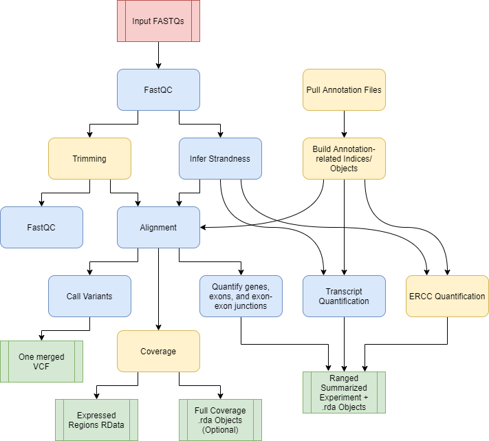
Functional workflow. Yellow coloring denotes steps which are optional or not always performed.
SPEAQeasy Outputs
SPEAQeasy produces RangedSummarizedExperiment objects with raw and normalized counts for each feature type: genes, exons, exon-exon junctions, and transcripts.
For human samples, variant calling is performed at a list of highly variables sites. A single VCF file is generated, containing genotype calls for all samples. This estalishes a sufficiently unique profile for each sample which can be compared against pre-sequencing genotype calls to resolve potential identity issues.
Optionally, BigWig coverage files by strand, and averaged across strands, are produced. An additional step utilizes the derfinder package to compute expressed regions, a precursor to analyses finding differentially expressed regions (DERs).
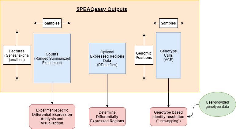
Main SPEAQeasy outputs of interest.
Installation and Set-up
First, clone the SPEAQeasy repository.
SPEAQeasy dependencies can be managed with docker, involving a fairly quick installation that is reproducible regardless of the computing environment. For those who are able to use docker, SPEAQeasy can be installed with:
If you do not have access to docker on your machine, SPEAQeasy can be installed with:
Please note that installation with docker is recommended if available, and that “local” installation can take quite some time, as all dependencies are built from source. Installing and running SPEAQeasy is not required for this workshop, but is demonstrated to familiarize participants with the process. The workshop files include outputs from SPEAQeasy, which can be used later for the example differential expression analysis.
Choose a “main” script as appropriate for your particular set-up. “Main” scripts and associated configuration files exist for SLURM-managed computing clusters, SGE-managed clusters, local machines, and the JHPCE cluster.
| Environment | “Main” script | Config file |
|---|---|---|
| SLURM cluster | run_pipeline_slurm.sh | conf/slurm.config or conf/docker_slurm.config |
| SGE cluster | run_pipeline_sge.sh | conf/sge.config or conf/docker_sge.config |
| Local machine | run_pipeline_local.sh | conf/local.config or conf/docker_local.config |
| JHPCE cluster | run_pipeline_jhpce.sh | conf/jhpce.config |
Within the main script, you can configure arguments specific to the experiment, such as the reference organism, pairing of samples, and where to place output files, among other specifications.
When running SPEAQeasy on a cluster (i.e. SLURM, SGE, or JHPCE users), it is recommended you submit the pipeline as a job, using the command appropriate for your cluster. For those running SPEAQeasy locally, the main script can be executed directly.
#  SLURM-managed clusters
sbatch run_pipeline_slurm.sh

#  SGE-managed clusters
qsub run_pipeline_sge.sh

#  local machines
bash run_pipeline_local.sh

#  The JHPCE cluster
qsub run_pipeline_jhpce.sh
Here’s an example of such a file.
## Root for our example files
example_files <- system.file(
    "extdata",
    "SPEAQeasy-example",
    package = "SPEAQeasyWorkshop2020"
)

## Read in the actual bash script used to run SPEAQeasy with the
## data from SPEAQeasy-example
cat(paste0(readLines(
    file.path(example_files, "pipeline_outputs", "run_pipeline_jhpce.sh")
), "\n"))
#> #!/bin/bash
#>  #$ -l bluejay,mem_free=60G,h_vmem=60G,h_fsize=800G
#>  #$ -N SPEAQeasy_ex
#>  #$ -o ./SPEAQeasy_ex.log
#>  #$ -e ./SPEAQeasy_ex.log
#>  #$ -cwd
#>
#>  module load nextflow
#>  export _JAVA_OPTIONS="-Xms8g -Xmx10g"
#>
#>  nextflow /dcl01/lieber/ajaffe/Nick/RNAsp/main.nf \
#>      --sample "paired" \
#>      --reference "hg38" \
#>      --strand "reverse" \
#>      --coverage \
#>      --annotation "/dcl01/lieber/ajaffe/Nick/RNAsp/Annotation" \
#>      -with-report execution_reports/JHPCE_run.html \
#>      -with-dag execution_DAGs/JHPCE_run.html \
#>      -profile jhpce \
#>      -w "/dcl01/lieber/ajaffe/lab/RNAsp_work/runs" \
#>      --input "/dcl01/lieber/ajaffe/lab/SPEAQeasy-example/sample_selection" \
#>      --output "/dcl01/lieber/ajaffe/lab/SPEAQeasy-example/pipeline_outputs"
#>
#>  #  Produces a report for each sample tracing the pipeline steps
#>  #  performed (can be helpful for debugging).
#>  #
#>  #  Note that the reports are generated from the output log produced in the above
#>  #  section, and so if you rename the log, you must also pass replace the filename
#>  #  in the bash call below.
#>  #echo "Generating per-sample logs for debugging..."
#>  #bash /dcl01/lieber/ajaffe/Nick/RNAsp/scripts/generate_logs.sh $PWD/SPEAQeasy_output.log
Examining SPEAQeasy outputs
Let’s take a look at one of the major outputs from SPEAQeasy- the RangedSummarizedExperiment containing gene counts.
library("SummarizedExperiment")
library("jaffelab") # GitHub: LieberInstitute/jaffelab
#  Load the RSE containing gene counts
load(
    file.path(
        example_files,
        "pipeline_outputs",
        "count_objects",
        "rse_gene_Jlab_experiment_n42.Rdata"
    ),
    verbose = TRUE
)
#> Loading objects:
#>   rse_gene

#  Print an overview
rse_gene
#> class: RangedSummarizedExperiment
#> dim: 60609 42
#> metadata(0):
#> assays(1): counts
#> rownames(60609): ENSG00000223972.5 ENSG00000227232.5 ...
#>   ENSG00000210195.2 ENSG00000210196.2
#> rowData names(10): Length gencodeID ... NumTx gencodeTx
#> colnames(42): R13896_H7JKMBBXX R13903_HCTYLBBXX ... R15120_HFY2MBBXX
#>   R15134_HFFGHBBXX
#> colData names(61): SAMPLE_ID FQCbasicStats ...
#>   gene_Unassigned_Ambiguity rRNA_rate

#  Check out the metrics SPEAQeasy collected for each sample, including stats
#  from FastQC, trimming, and alignment
colnames(colData(rse_gene))
#>  [1] "SAMPLE_ID"                          "FQCbasicStats"
#>  [3] "perBaseQual"                        "perTileQual"
#>  [5] "perSeqQual"                         "perBaseContent"
#>  [7] "GCcontent"                          "Ncontent"
#>  [9] "SeqLengthDist"                      "SeqDuplication"
#> [11] "OverrepSeqs"                        "AdapterContent"
#> [13] "KmerContent"                        "SeqLength_R1"
#> [15] "percentGC_R1"                       "phred20-21_R1"
#> [17] "phred48-49_R1"                      "phred76-77_R1"
#> [19] "phred100-101_R1"                    "phredGT30_R1"
#> [21] "phredGT35_R1"                       "Adapter50-51_R1"
#> [23] "Adapter70-71_R1"                    "Adapter90_R1"
#> [25] "SeqLength_R2"                       "percentGC_R2"
#> [27] "phred20-21_R2"                      "phred48-49_R2"
#> [29] "phred76-77_R2"                      "phred100-101_R2"
#> [31] "phredGT30_R2"                       "phredGT35_R2"
#> [33] "Adapter50-51_R2"                    "Adapter70-71_R2"
#> [35] "Adapter90_R2"                       "bamFile"
#> [37] "trimmed"                            "numReads"
#> [39] "numMapped"                          "numUnmapped"
#> [41] "overallMapRate"                     "concordMapRate"
#> [43] "totalMapped"                        "mitoMapped"
#> [45] "mitoRate"                           "totalAssignedGene"
#> [47] "gene_Assigned"                      "gene_Unassigned_Unmapped"
#> [49] "gene_Unassigned_Read_Type"          "gene_Unassigned_Singleton"
#> [51] "gene_Unassigned_MappingQuality"     "gene_Unassigned_Chimera"
#> [53] "gene_Unassigned_FragmentLength"     "gene_Unassigned_Duplicate"
#> [55] "gene_Unassigned_MultiMapping"       "gene_Unassigned_Secondary"
#> [57] "gene_Unassigned_NonSplit"           "gene_Unassigned_NoFeatures"
#> [59] "gene_Unassigned_Overlapping_Length" "gene_Unassigned_Ambiguity"
#> [61] "rRNA_rate"

#  View the "top left corner" of the counts assay, containing counts for a few
#  genes and a few samples
corner(assays(rse_gene)$counts)
#>                   R13896_H7JKMBBXX R13903_HCTYLBBXX R13904_H7K5NBBXX
#> ENSG00000223972.5                0                0                0
#> ENSG00000227232.5               46               36               20
#> ENSG00000278267.1                8                3                0
#> ENSG00000243485.5                0                0                0
#> ENSG00000284332.1                0                0                0
#> ENSG00000237613.2                0                0                0
#>                   R13983_H7JKMBBXX R13985_H7JM5BBXX R13986_H7JM5BBXX
#> ENSG00000223972.5                0                0                0
#> ENSG00000227232.5              118               61               47
#> ENSG00000278267.1               13                4                8
#> ENSG00000243485.5                0                1                0
#> ENSG00000284332.1                0                0                0
#> ENSG00000237613.2                0                0                0

#  Examine what data is provided in the RSE object for each gene ("row")
head(rowData(rse_gene))
#> DataFrame with 6 rows and 10 columns
#>                      Length         gencodeID       ensemblID
#>                   <integer>       <character>     <character>
#> ENSG00000223972.5      1735 ENSG00000223972.5 ENSG00000223972
#> ENSG00000227232.5      1351 ENSG00000227232.5 ENSG00000227232
#> ENSG00000278267.1        68 ENSG00000278267.1 ENSG00000278267
#> ENSG00000243485.5      1021 ENSG00000243485.5 ENSG00000243485
#> ENSG00000284332.1       138 ENSG00000284332.1 ENSG00000284332
#> ENSG00000237613.2      1219 ENSG00000237613.2 ENSG00000237613
#>                                gene_type      Symbol  EntrezID       Class
#>                              <character> <character> <integer> <character>
#> ENSG00000223972.5 transcribed_unproces..     DDX11L1        NA       InGen
#> ENSG00000227232.5 unprocessed_pseudogene      WASH7P        NA       InGen
#> ENSG00000278267.1                  miRNA   MIR6859-1        NA       InGen
#> ENSG00000243485.5                 lncRNA MIR1302-2HG        NA       InGen
#> ENSG00000284332.1                  miRNA   MIR1302-2        NA       InGen
#> ENSG00000237613.2                 lncRNA     FAM138A        NA       InGen
#>                    meanExprs     NumTx              gencodeTx
#>                    <numeric> <integer>            <character>
#> ENSG00000223972.5 0.00347263         2 ENST00000456328.2;EN..
#> ENSG00000227232.5 1.57167877         1      ENST00000488147.1
#> ENSG00000278267.1 7.74437941         1      ENST00000619216.1
#> ENSG00000243485.5 0.01403484         2 ENST00000473358.1;EN..
#> ENSG00000284332.1 0.00000000         1      ENST00000607096.1
#> ENSG00000237613.2 0.00683033         2 ENST00000417324.1;EN..
Identifying sample swaps
Note: the original version is available here and was written by Josh Stolz and Louise Huuki.
In order to resolve the swaps to our best ability we need four data sets. Here we have load snpGeno_example which is from our TOPMed imputed genotype data, a phenotype data sheet (pd_example), a VCF file of the relevant SPEAQeasy output (SPEAQeasy), and our current genotype sample sheet (brain_sentrix). This file is available in the directory listed below.
load(file.path(example_files, "sample_selection", "snpsGeno_example.RData"),
    verbose = TRUE
)
#> Loading objects:
#>   snpsGeno_example
load(file.path(example_files, "sample_selection", "pd_example.Rdata"),
    verbose = TRUE
)
#> Loading objects:
#>   pd_example
Speaqeasy <-
    readVcf(
        file.path(
            example_files,
            "pipeline_outputs",
            "merged_variants",
            "mergedVariants.vcf.gz"
        ),
        genome = "hg38"
    )
brain_sentrix <-
    read.csv(file.path(example_files, "brain_sentrix_speaqeasy.csv"))
We can see that the genotype is represented in the form of 0s, 1s, and 2s. The rare 2s are a result of multiallelic SNPs and we will drop those. 0 represent the reference allele with ones representing the alternate. We can see the distribution below.
Geno_speaqeasy <- geno(Speaqeasy)$GT
table(Geno_speaqeasy)
#> Geno_speaqeasy
#>   ./.   0/1   0/2   1/1   2/2
#> 14096  7803     4  6018     9
Given this we convert we convert the Genotype data from SPEAQeasy to numeric data. The "./." were values that could not accurately be determined and are replaced with NA.
colnames_speaqeasy <- as.data.frame(colnames(Geno_speaqeasy))
colnames(colnames_speaqeasy) <- c("a")
samples <-
tidyr::separate(colnames_speaqeasy,
a,
into = c("a", "b", "c"),
sep = "_"
)
#> Warning: Expected 3 pieces. Additional pieces discarded in 42 rows [1, 2, 3, 4,
#> 5, 6, 7, 8, 9, 10, 11, 12, 13, 14, 15, 16, 17, 18, 19, 20, ...].
samples <- paste0(samples$a, "_", samples$b)
samples <- as.data.frame(samples)
colnames(Geno_speaqeasy) <- samples$samples
Geno_speaqeasy[Geno_speaqeasy == "./."] <- NA
Geno_speaqeasy[Geno_speaqeasy == "0/0"] <- 0
Geno_speaqeasy[Geno_speaqeasy == "0/1"] <- 1
Geno_speaqeasy[Geno_speaqeasy == "1/1"] <- 2
class(Geno_speaqeasy) <- "numeric"
#> Warning in class(Geno_speaqeasy) <- "numeric": NAs introduced by coercion
corner(Geno_speaqeasy)
#> R14030_H7K5NBBXX R14184_H7K5NBBXX R13904_H7K5NBBXX
#> chr1:4712657_G/A 2 1 2
#> chr1:7853370_G/A NA NA NA
#> chr1:9263851_G/A NA NA 1
#> chr1:13475857_T/C NA NA NA
#> chr1:15289643_G/A NA NA NA
#> chr1:15341780_G/A NA NA NA
#> R14296_H7JLCBBXX R14247_HF3JYBBXX R15093_HFY2MBBXX
#> chr1:4712657_G/A 1 1 2
#> chr1:7853370_G/A NA NA NA
#> chr1:9263851_G/A 1 1 NA
#> chr1:13475857_T/C NA NA NA
#> chr1:15289643_G/A NA NA NA
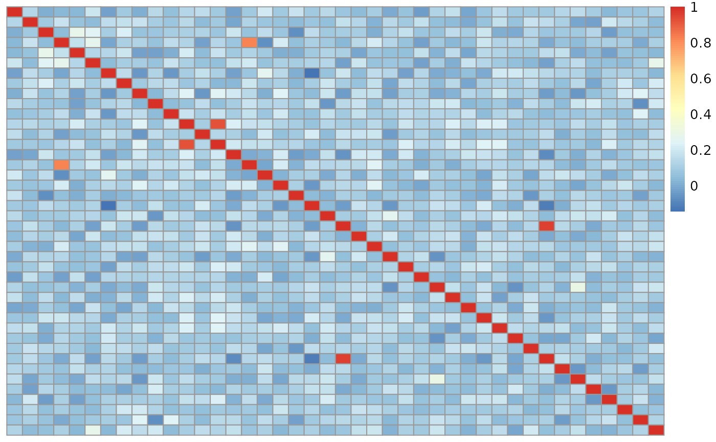
#> chr1:15341780_G/A NA NA 1We then make a correlation matrix to find the possible mismatches between samples.
speaqeasy_Cor <- cor(Geno_speaqeasy, use = "pairwise.comp")
corner(speaqeasy_Cor)
#>                  R14030_H7K5NBBXX R14184_H7K5NBBXX R13904_H7K5NBBXX
#> R14030_H7K5NBBXX       1.00000000       0.13507812       0.01657484
#> R14184_H7K5NBBXX       0.13507812       1.00000000       0.09347004
#> R13904_H7K5NBBXX       0.01657484       0.09347004       1.00000000
#> R14296_H7JLCBBXX       0.03106472       0.18748043       0.04958385
#> R14247_HF3JYBBXX       0.03384912       0.07080491       0.28798955
#> R15093_HFY2MBBXX       0.18938568       0.04720309       0.25477682
#>                  R14296_H7JLCBBXX R14247_HF3JYBBXX R15093_HFY2MBBXX
#> R14030_H7K5NBBXX       0.03106472       0.03384912       0.18938568
#> R14184_H7K5NBBXX       0.18748043       0.07080491       0.04720309
#> R13904_H7K5NBBXX       0.04958385       0.28798955       0.25477682
#> R14296_H7JLCBBXX       1.00000000       0.16653808       0.27251010
#> R14247_HF3JYBBXX       0.16653808       1.00000000       0.14097339
#> R15093_HFY2MBBXX       0.27251010       0.14097339       1.00000000
Here in the heatmap below we can see that several points do not correlate with themselves in a symmetrical matrix. This could be mismatches, but it also could be a result of a brain being sequenced twice. We will dig more into this later on.
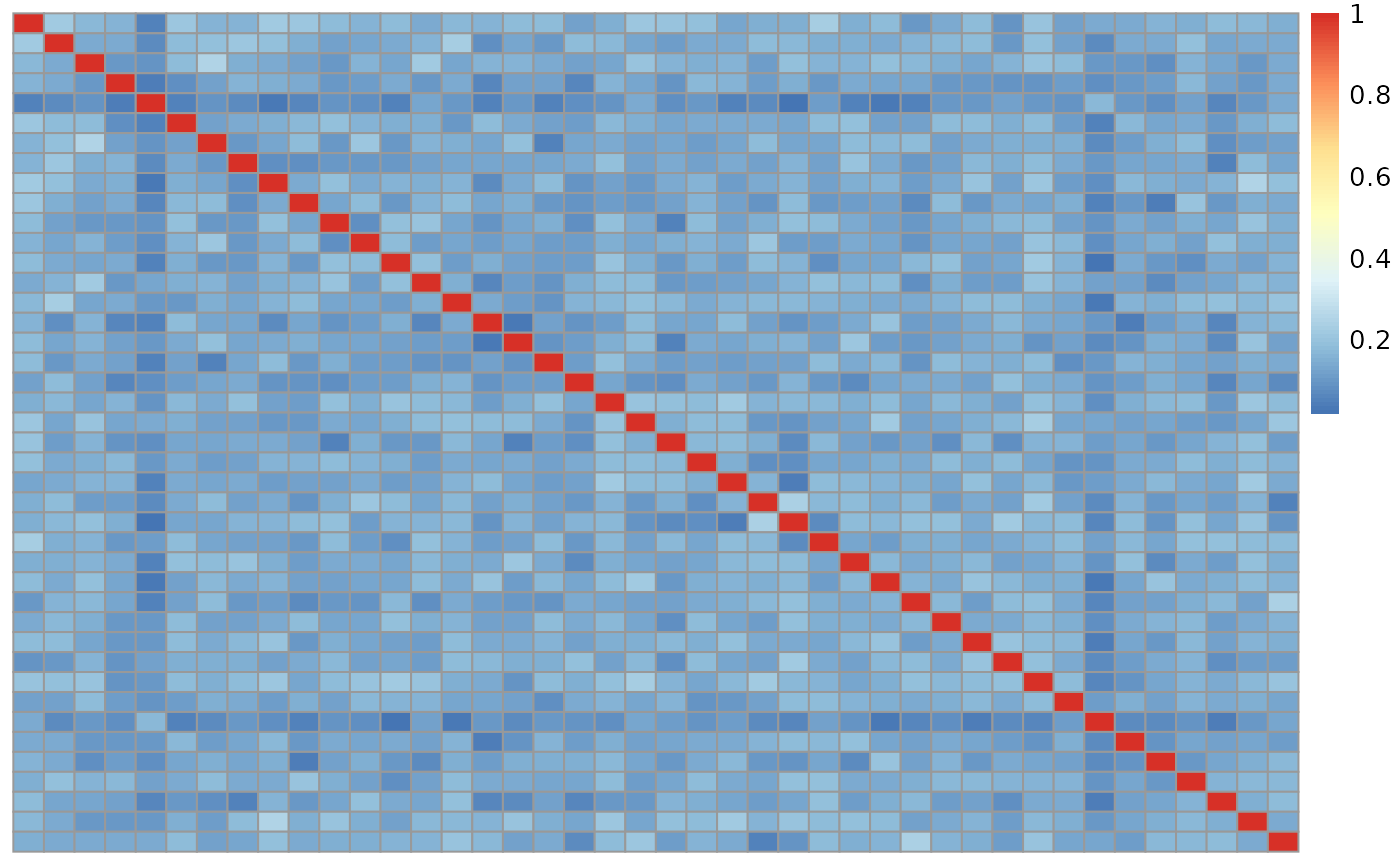
We repeat the process for the genotype data from TOPMed. First creating our numeric data for the genotypes.
#> Geno_example
#>  0|0  0|1  1|0  1|1
#> 9656 6956 7185 7535
#>                   4463344375_R01C01 4463344375_R01C02 4572348848_R01C02
#> 4463344375_R01C01        1.00000000        0.21736687        0.17615291
#> 4463344375_R01C02        0.21736687        1.00000000        0.13803954
#> 4572348848_R01C02        0.17615291        0.13803954        1.00000000
#> 4572348855_R01C02        0.16590842        0.14670605        0.10600440
#> 5535549043_R01C01        0.05367081        0.07697879        0.09356496
#> 5535506145_R01C01        0.21189898        0.18114194        0.17829111
#>                   4572348855_R01C02 5535549043_R01C01 5535506145_R01C01
#> 4463344375_R01C01        0.16590842        0.05367081        0.21189898
#> 4463344375_R01C02        0.14670605        0.07697879        0.18114194
#> 4572348848_R01C02        0.10600440        0.09356496        0.17829111
#> 4572348855_R01C02        1.00000000        0.04874508        0.08186958
#> 5535549043_R01C01        0.04874508        1.00000000        0.05331113
#> 5535506145_R01C01        0.08186958        0.05331113        1.00000000
In this case the data only appears to have samples that match themselves. However there is the potential for a second kind of error where a brain has two samples, however the do not match each other.
We will next compare the correlation between the SPEAQeasy samples and the TOPMed samples. In order to do this we need to subset the genotypes for only SNPs that are common between the two. We can see that we have 662 snps common between the 42 samples.
Geno_speaqeasy_subset <-
    Geno_speaqeasy[rownames(Geno_speaqeasy) %in% rownames(Geno_example), ]
snpsGeno_subset <-
    Geno_example[rownames(Geno_example) %in% rownames(Geno_speaqeasy_subset), ]
dim(Geno_speaqeasy_subset)
#> [1] 662  42
dim(snpsGeno_subset)
#> [1] 662  42
As we did before we create a correlation matrix this time between the two data sets.
correlation_genotype_speaq <-
    cor(snpsGeno_subset, Geno_speaqeasy_subset, use = "pairwise.comp")
In order to dig into this further we will collapse the correlation matrices into a data table shown below.
## Convert to long format
corLong3 <-
    data.frame(cor = signif(as.numeric(correlation_genotype_speaq), 3))
corLong3$rowSample <-
    rep(colnames(snpsGeno_example), times = ncol(snpsGeno_example))
corLong3$colSample <-
    rep(colnames(Geno_speaqeasy), each = ncol(Geno_speaqeasy))
Check the correlation between SPEAQeasy and Genotype for mismatches and swaps.
brain_sentrix_present <-
    subset(brain_sentrix, ID %in% colnames(snpsGeno_example))

## Match across tables
speaqeasy_match_col <-
    match(corLong3$colSample, pd_example$SAMPLE_ID)
corLong3$colBrain <- pd_example$BrNum[speaqeasy_match_col]
brain_sentrix_match_row <-
    match(corLong3$rowSample, brain_sentrix_present$ID)
corLong3$rowBrain <-
    brain_sentrix_present$BrNum[brain_sentrix_match_row]

# Fails to match
corLong3[corLong3$rowBrain == corLong3$colBrain &
    corLong3$cor < .8, ]
#>           cor         rowSample        colSample colBrain rowBrain
#> 165   0.00962 9373408026_R01C01 R14296_H7JLCBBXX   Br2473   Br2473
#> 425   0.11600 5535549043_R01C01 R14129_HCTYLBBXX   Br1652   Br1652
#> 432   0.11800 6017049081_R01C02 R14129_HCTYLBBXX   Br1652   Br1652
#> 498  -0.04270 9373406026_R02C01 R14222_H7JHNBBXX   Br2275   Br2275
#> 582  -0.03790 9373406026_R02C01 R13997_H7JHNBBXX   Br2275   Br2275
#> 669   0.08540 9373408026_R01C01 R14077_HCTYLBBXX   Br2473   Br2473
#> 917   0.04020 9373406026_R01C01 R14290_H7L3FBBXX   Br2260   Br2260
#> 1463  0.05050 9373406026_R01C01 R14071_HF3JYBBXX   Br2260   Br2260
#> 1697  0.76500 3998646040_R06C01 R14017_HF5JNBBXX   Br5190   Br5190

# Mismatches
corLong3[!corLong3$rowBrain == corLong3$colBrain &
    corLong3$cor > .8, ]
#>        cor         rowSample        colSample colBrain rowBrain
#> 161  0.865 9373406026_R01C01 R14296_H7JLCBBXX   Br2473   Br2260
#> 665  0.815 9373406026_R01C01 R14077_HCTYLBBXX   Br2473   Br2260
#> 921  0.866 9373408026_R01C01 R14290_H7L3FBBXX   Br2260   Br2473
#> 1467 0.915 9373408026_R01C01 R14071_HF3JYBBXX   Br2260   Br2473
We can see from this from this analysis there are a few swaps present between RNA and DNA samples here. We can categorize them as simple and complex sample swaps. Because the two Br2275 do not match each other and also match nothing else we will be forced to consider this a complex swap and drop the sample. In the case of Br2473 it is a simple swap with Br2260 in both cases. This can be amended by swapping with in the phenotype data sheet manually. Now we have our accurate data outputs and will need to fix our ranged summarized experiment object for our SPEAQeasy data.
## drop sample from rse with SPEAQeasy data
ids <- pd_example$SAMPLE_ID[pd_example$BrNum == "Br2275"]
rse_gene <- rse_gene[, !rse_gene$SAMPLE_ID == ids[1]]
rse_gene <- rse_gene[, !rse_gene$SAMPLE_ID == ids[2]]

# resolve swaps and drops in pd_example
pd_example <- pd_example[!pd_example$SAMPLE_ID == ids[1], ]
pd_example <- pd_example[!pd_example$SAMPLE_ID == ids[2], ]
ids2 <- pd_example$SAMPLE_ID[pd_example$BrNum == "Br2260"]
ids3 <- pd_example$SAMPLE_ID[pd_example$BrNum == "Br2473"]
pd_example$SAMPLE_ID[pd_example$Sample_ID == ids2] <- "Br2473"
pd_example$SAMPLE_ID[pd_example$Sample_ID == ids3] <- "Br2260"

# reorder phenotype data by the sample order present in the 'rse_gene' object
pd_example <-
    pd_example[match(rse_gene$SAMPLE_ID, pd_example$SAMPLE_ID), ]

# add important colData to 'rse_gene'
rse_gene$BrainRegion <- pd_example$BrainRegion
rse_gene$Race <- pd_example$Race
rse_gene$PrimaryDx <- pd_example$PrimaryDx
rse_gene$Sex <- pd_example$Sex
rse_gene$AgeDeath <- pd_example$AgeDeath

# add correct BrNum to colData for rse_gene
colData(rse_gene)$BrNum <- pd_example$BrNum
We can then save the gene counts with the resolved sample swaps.
## You can then save the data
save(rse_gene, file = "rse_speaqeasy.RData")
DE Analysis
Note: the original version is available here and was written by Josh Stolz.
Resuming
In case that you skipped the previous section, you can load the data for the differential expression part with the following code.
## Root for our example files
example_files <- system.file(
    "extdata",
    "SPEAQeasy-example",
    package = "SPEAQeasyWorkshop2020"
)

## Load the file
load(file.path(example_files, "rse_speaqeasy.RData", verbose = TRUE))
The following analysis explores a RangedSummarizedExperiment object from the SPEAQeasy pipeline (Eagles, Burke, Leonard, et al., 2020). Note that we will use a modified version of the object, which resolved sample identity issues which were present in the raw output from SPEAQeasy. This object also includes phenotype data added after resolving identity issues. Though SPEAQeasy produces objects for several feature types (genes, exons, exon-exon junctions), we will demonstrate an example analysis for just genes. We will perform differential expression across some typical variables of interest (e.g. sex, age, race) and show how to perform principal component analysis (PCA) and visualize findings with plots.
Statistics PCs
Here we are using principal component analysis to control for the listed variables impact on expression. Later on, this could added into our linear model.
## Select variables of interest
col_names <- c(
    "trimmed",
    "numReads",
    "numMapped",
    "numUnmapped",
    "overallMapRate",
    "concordMapRate",
    "totalMapped",
    "mitoMapped",
    "mitoRate",
    "totalAssignedGene"
)
set.seed(20201006)

## Reduce these variables to one PC
statsPca <- prcomp(as.data.frame(colData(rse_gene)[, col_names]))
rse_gene$PC <- statsPca$x[, 1]
getPcaVars(statsPca)[1]
#> [1] 87.3
Stats vs. diagnosis and brain region
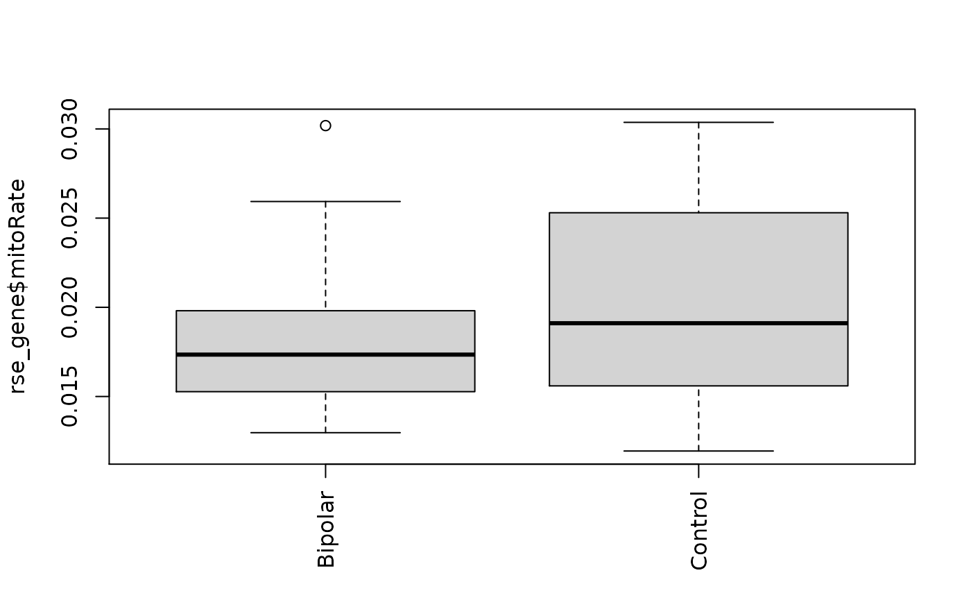
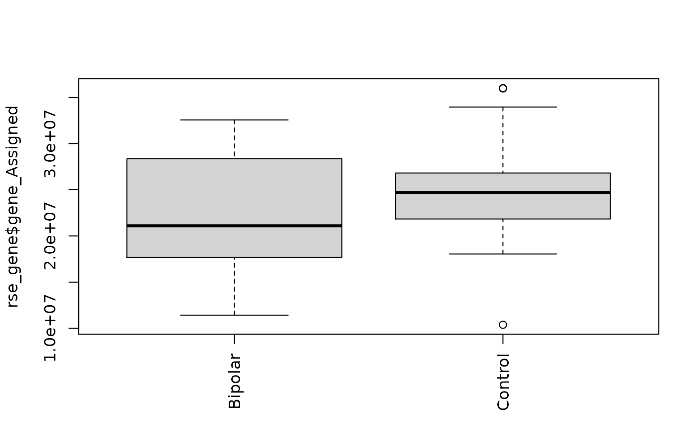
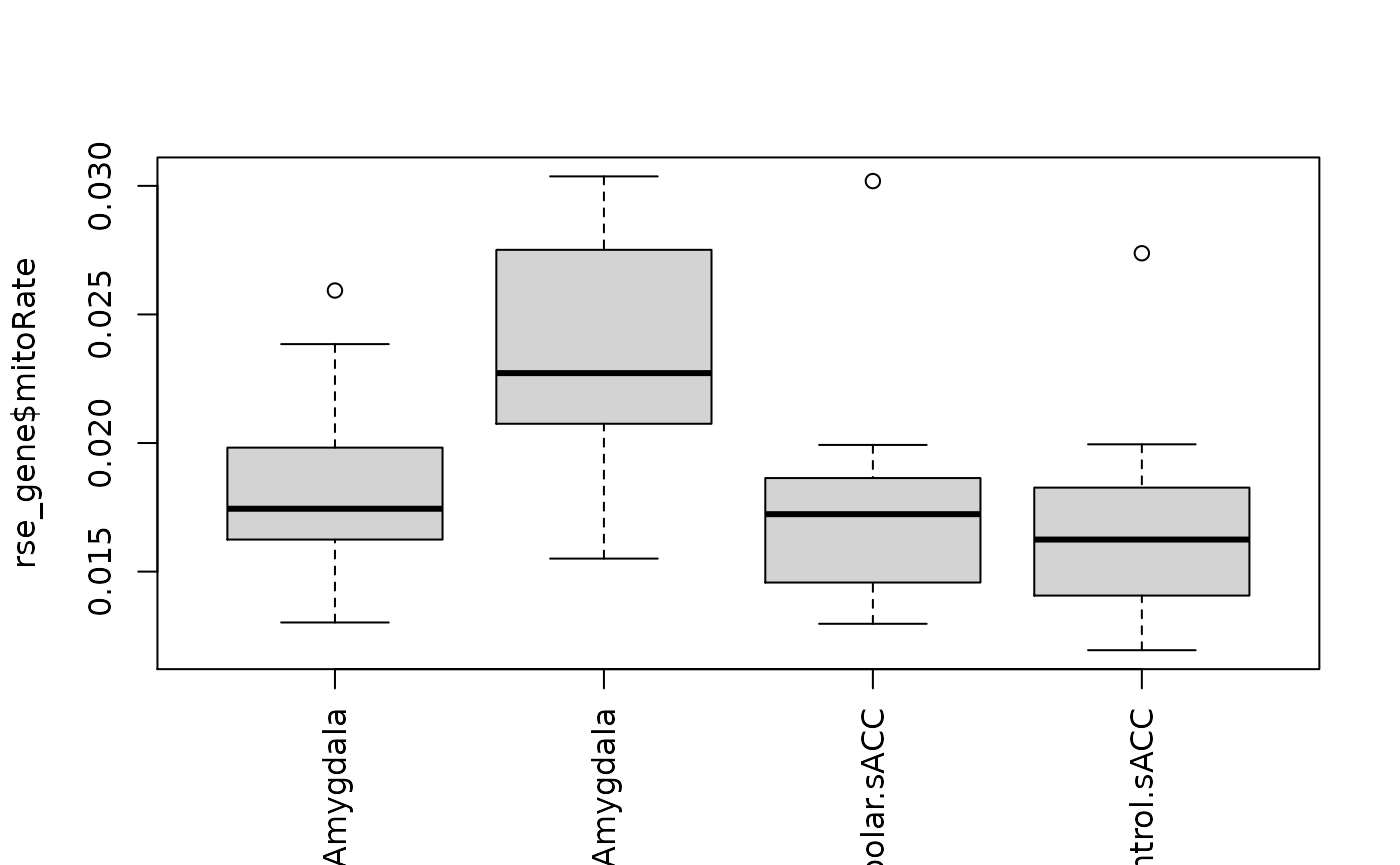
Here we explore the relationship between some quality control covariates produced by SPEAQeasy against phenotype data that we have on the samples such as brain region, primary diagnosis and race.
## We only have one race here
table(rse_gene$Race)
#>
#> CAUC
#>   40

# Display box plots here
boxplot(rse_gene$rRNA_rate ~ rse_gene$BrainRegion, xlab = "")
boxplot(rse_gene$mitoRate ~ rse_gene$BrainRegion, xlab = "")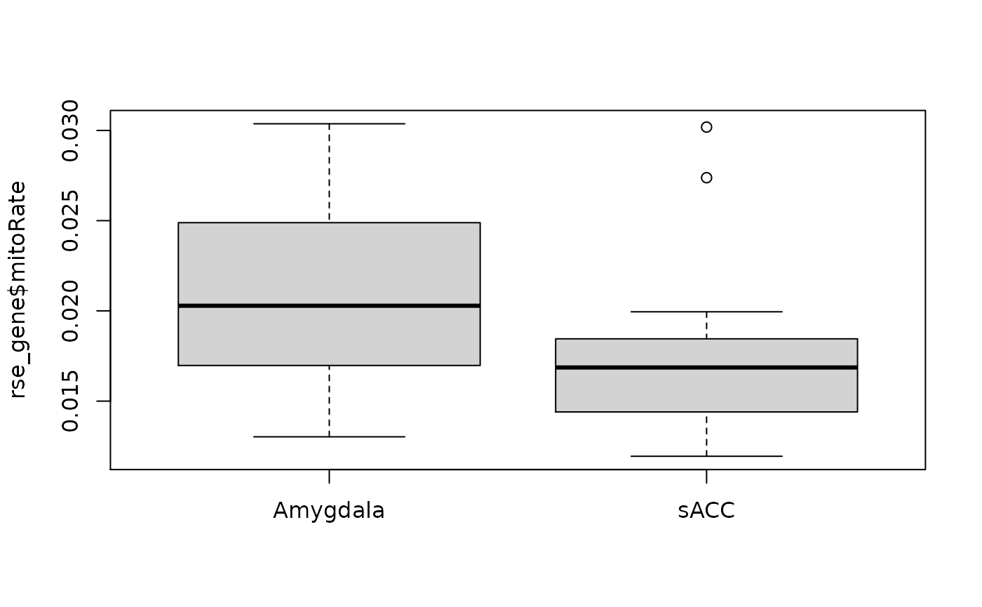
boxplot(rse_gene$gene_Assigned ~ rse_gene$BrainRegion, xlab = "")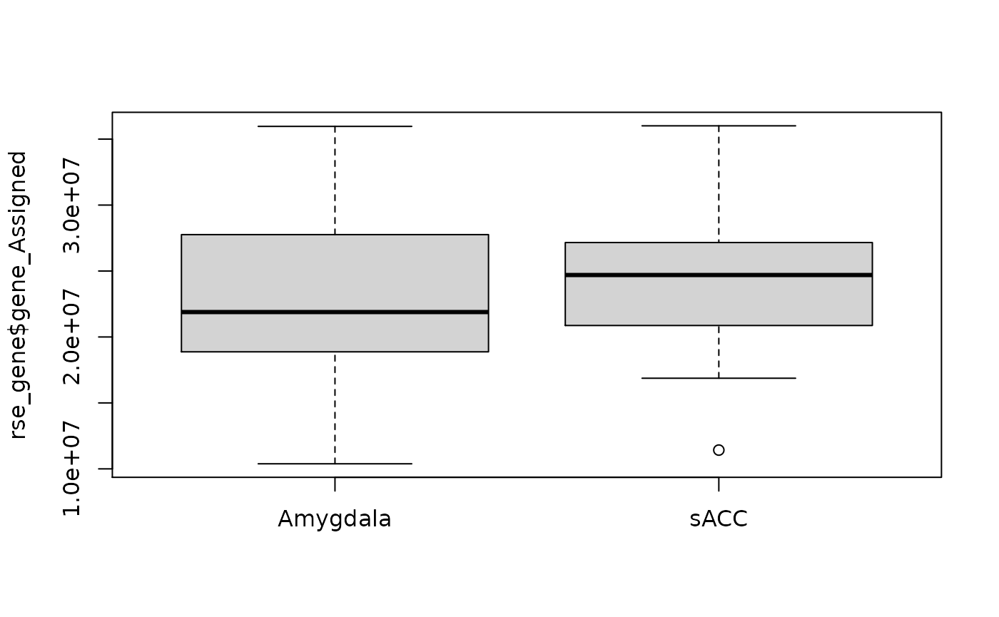
boxplot(rse_gene$mitoRate ~ rse_gene$PrimaryDx,
    las = 3,
    xlab = ""
)
boxplot(rse_gene$gene_Assigned ~ rse_gene$PrimaryDx,
    las = 3,
    xlab = ""
)
boxplot(
    rse_gene$mitoRate ~ rse_gene$PrimaryDx + rse_gene$BrainRegion,
    las = 3,
    xlab = ""
)
boxplot(
    rse_gene$gene_Assigned ~ rse_gene$PrimaryDx + rse_gene$BrainRegion,
    las = 3,
    xlab = ""
)
Explore and visualize gene expression
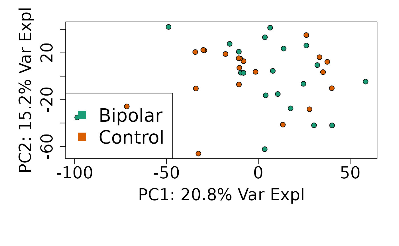
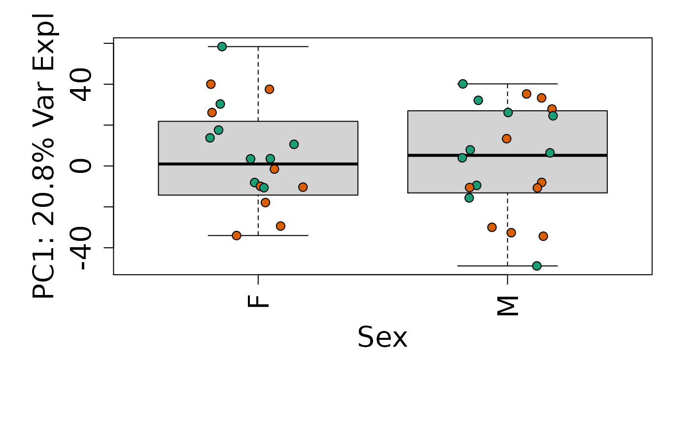
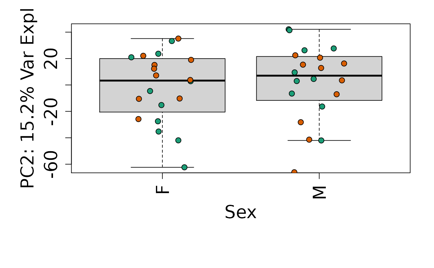
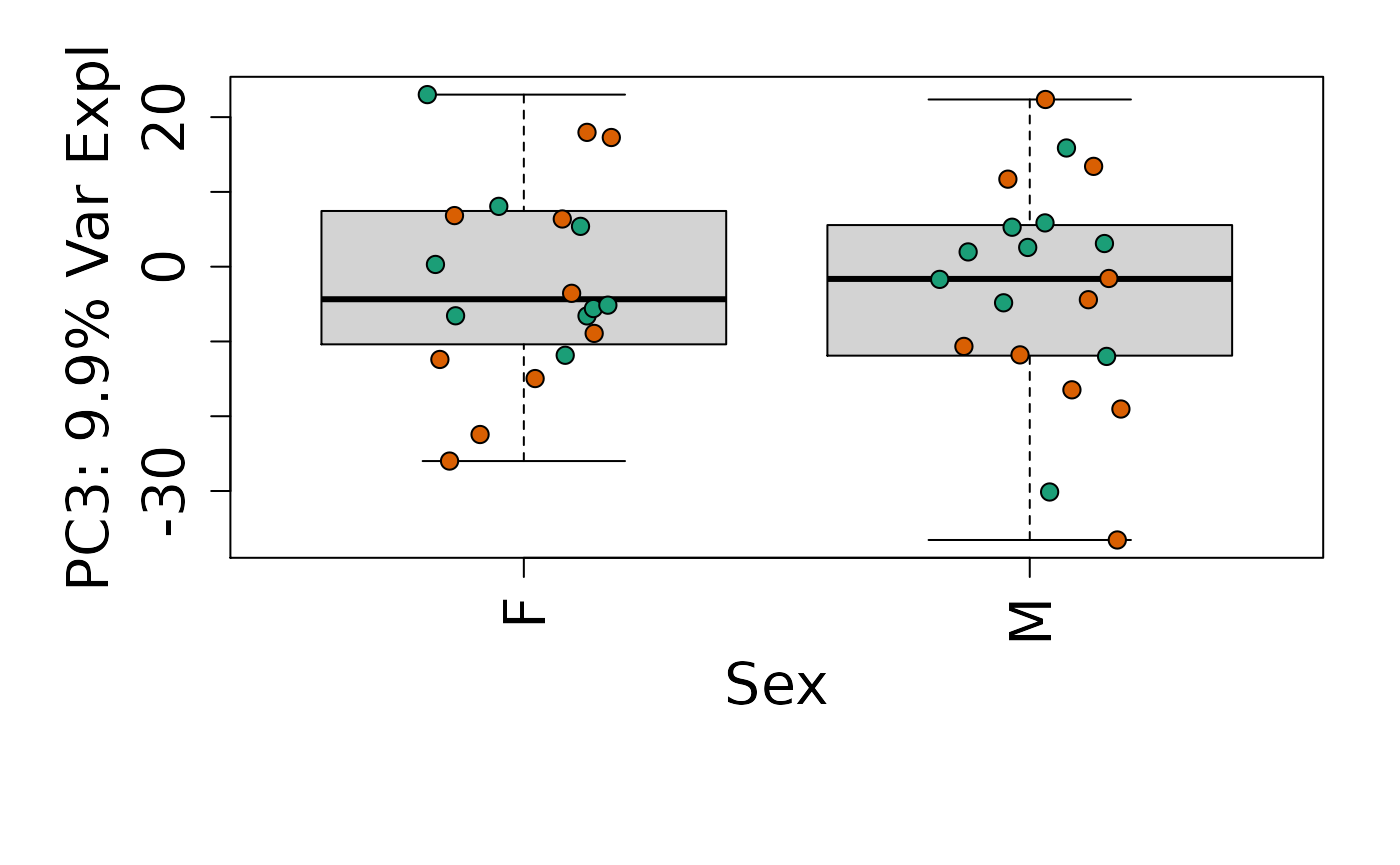
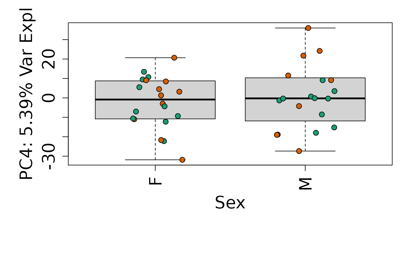
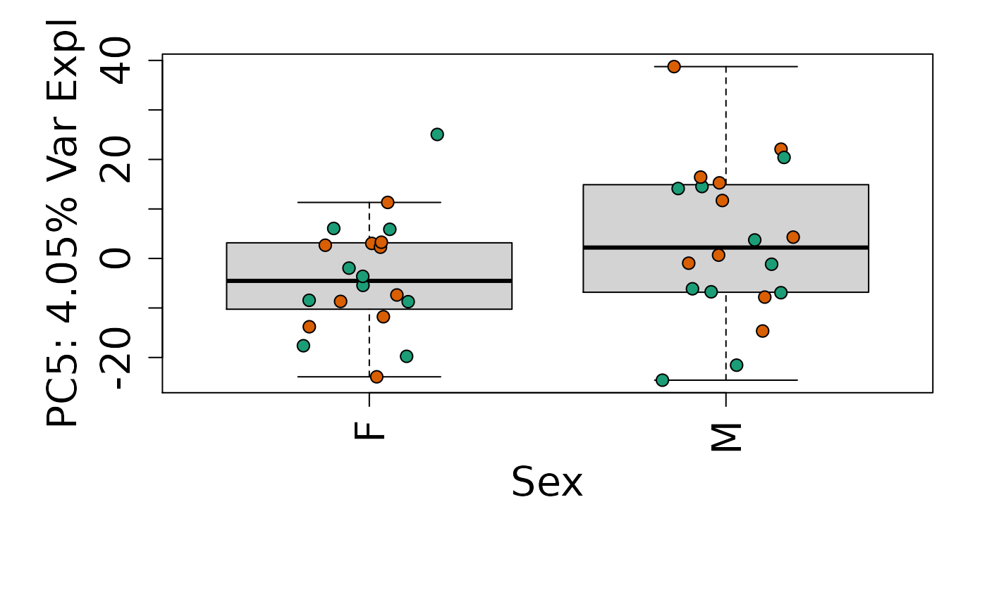
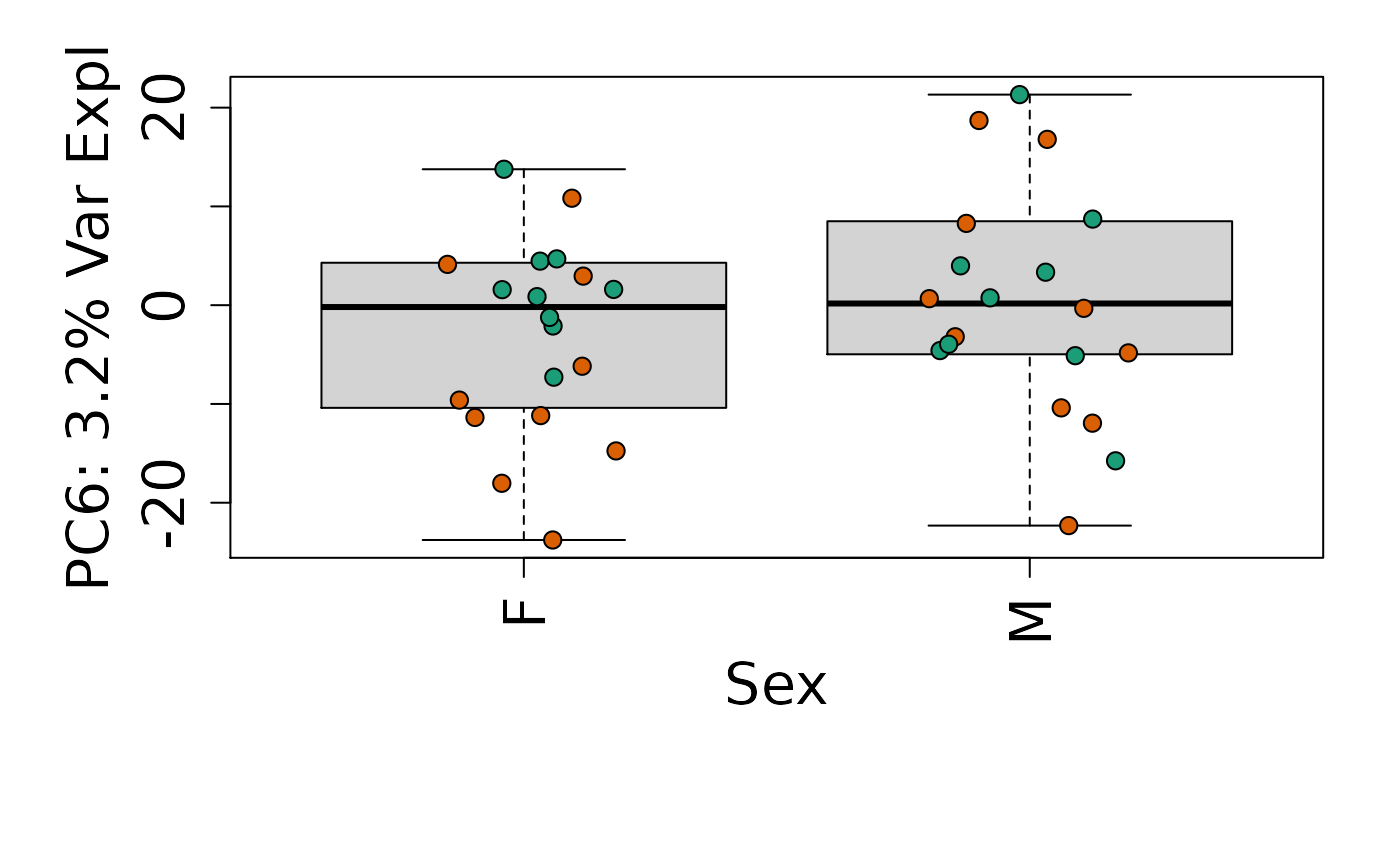
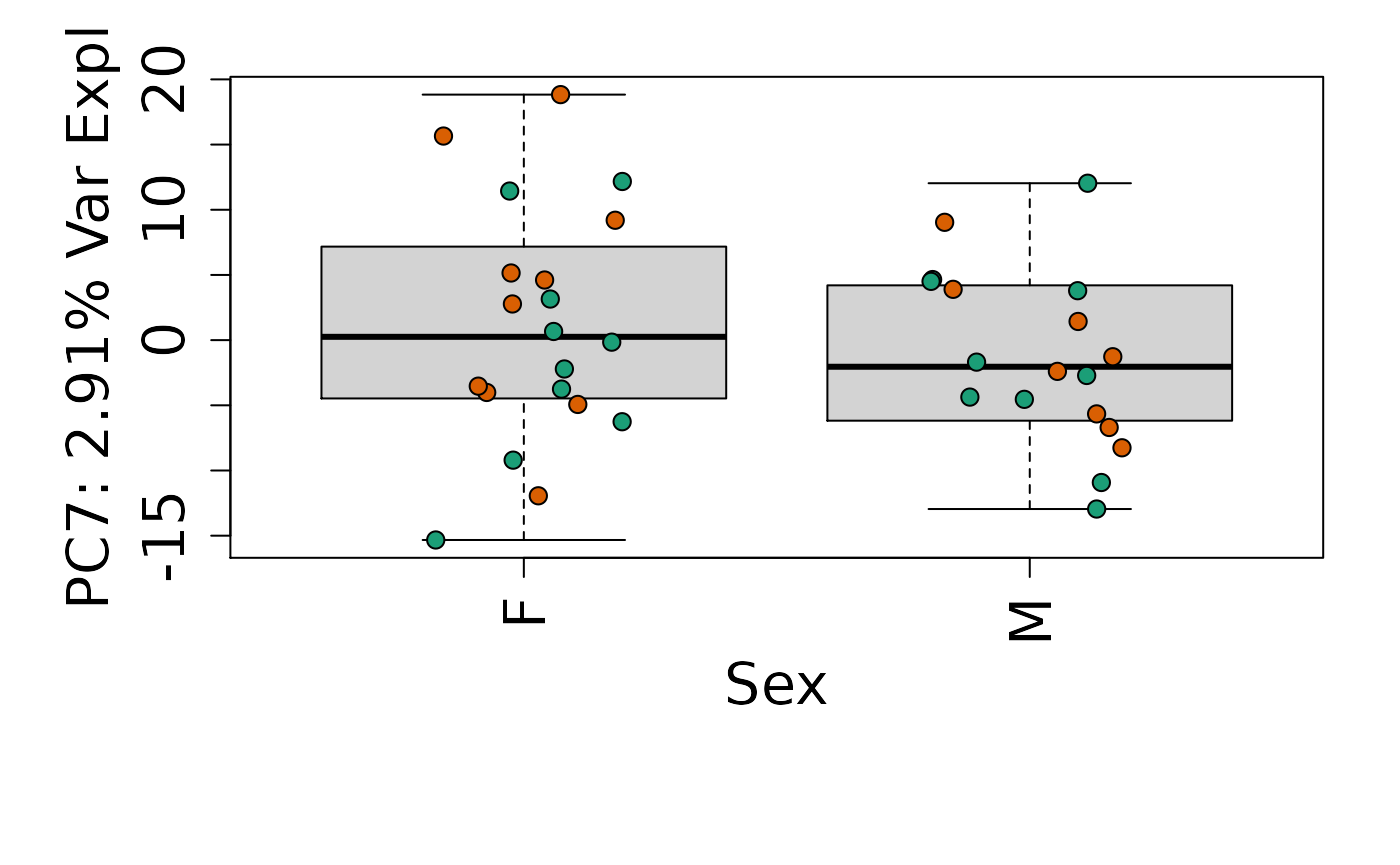
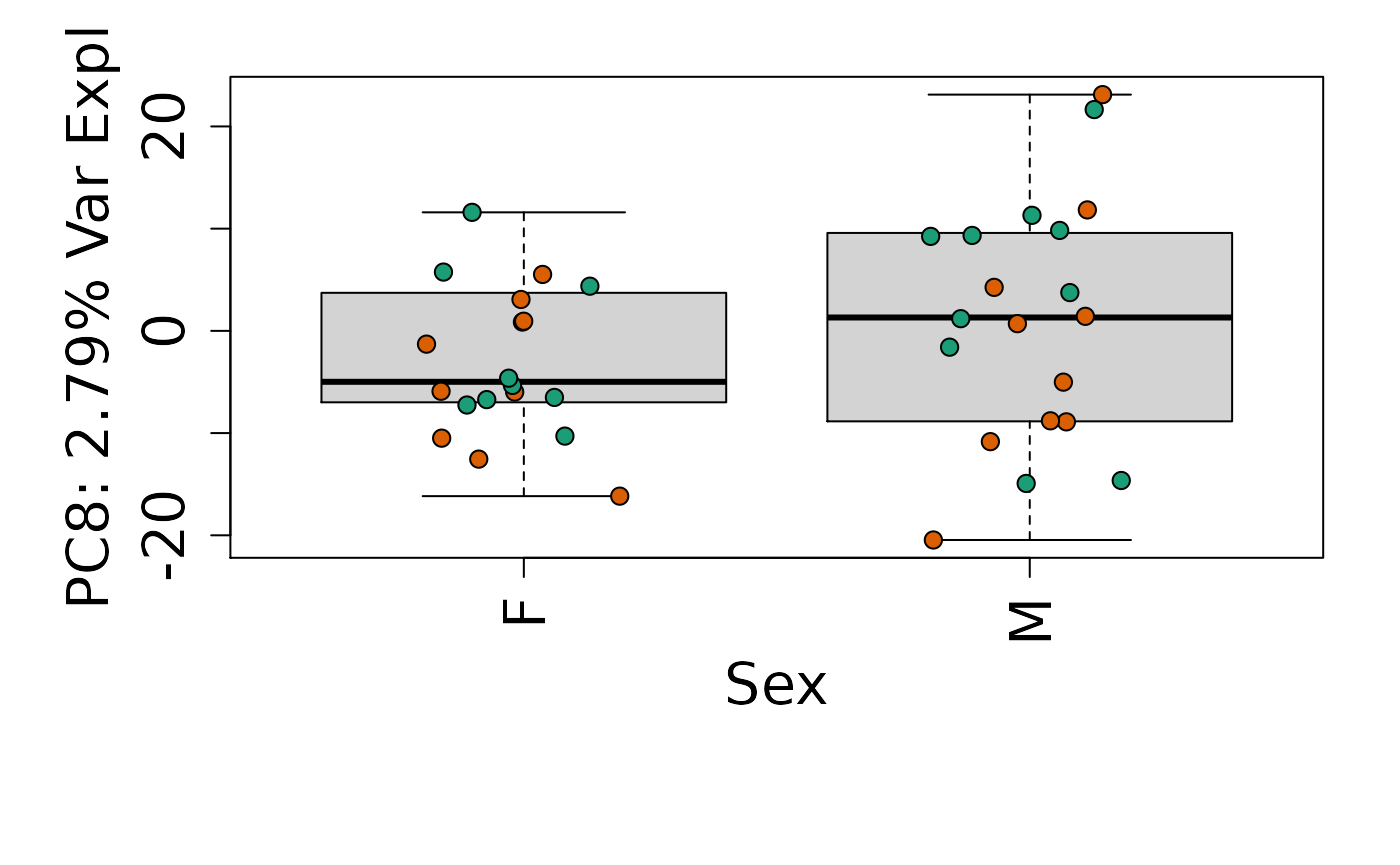
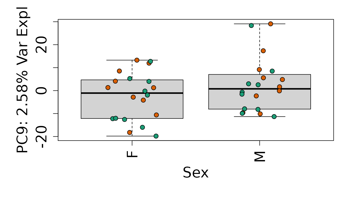
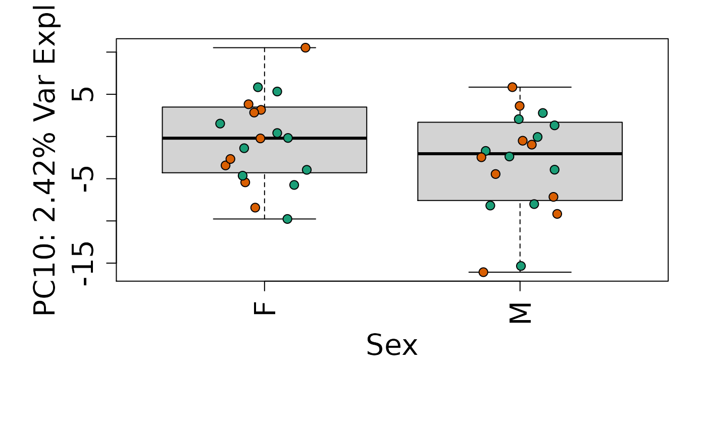
We can next explore overall patterns in the gene expression of our samples by visualizing the top principal components from the gene expression count data. For example, by visualizing the case-control samples in PC1 versus PC2. We can also check other covariates such as sex and brain region across the top 10 PCs.
# Filter for expressed
rse_gene <- rse_gene[rowMeans(getRPKM(rse_gene, "Length")) > 0.2, ]

# Explore gene expression
geneExprs <- log2(getRPKM(rse_gene, "Length") + 1)
set.seed(20201006)
pca <- prcomp(t(geneExprs))
pca_vars <- getPcaVars(pca)
pca_vars_lab <- paste0(
    "PC", seq(along = pca_vars), ": ",
    pca_vars, "% Var Expl"
)

# Group together code for generating plots of interest
set.seed(20201006)
par(
    mar = c(8, 6, 2, 2),
    cex.axis = 1.8,
    cex.lab = 1.8
)
palette(brewer.pal(4, "Dark2"))

# PC1 vs. PC2
plot(
    pca$x,
    pch = 21,
    bg = factor(rse_gene$PrimaryDx),
    cex = 1.2,
    xlab = pca_vars_lab[1],
    ylab = pca_vars_lab[2]
)
legend(
    "bottomleft",
    levels(rse_gene$PrimaryDx),
    col = 1:2,
    pch = 15,
    cex = 2
)
# By sex
for (i in 1:10) {
    boxplot(
        pca$x[, i] ~ rse_gene$Sex,
        ylab = pca_vars_lab[i],
        las = 3,
        xlab = "Sex",
        outline = FALSE
    )
    points(
        pca$x[, i] ~ jitter(as.numeric(factor(rse_gene$Sex))),
        pch = 21,
        bg = rse_gene$PrimaryDx,
        cex = 1.2
    )
}
# By brain region
for (i in 1:10) {
    boxplot(
        pca$x[, i] ~ rse_gene$BrainRegion,
        ylab = pca_vars_lab[i],
        las = 3,
        xlab = "Brain Region",
        outline = FALSE
    )
    points(
        pca$x[, i] ~ jitter(as.numeric(factor(
            rse_gene$BrainRegion
        ))),
        pch = 21,
        bg = rse_gene$PrimaryDx,
        cex = 1.2
    )
}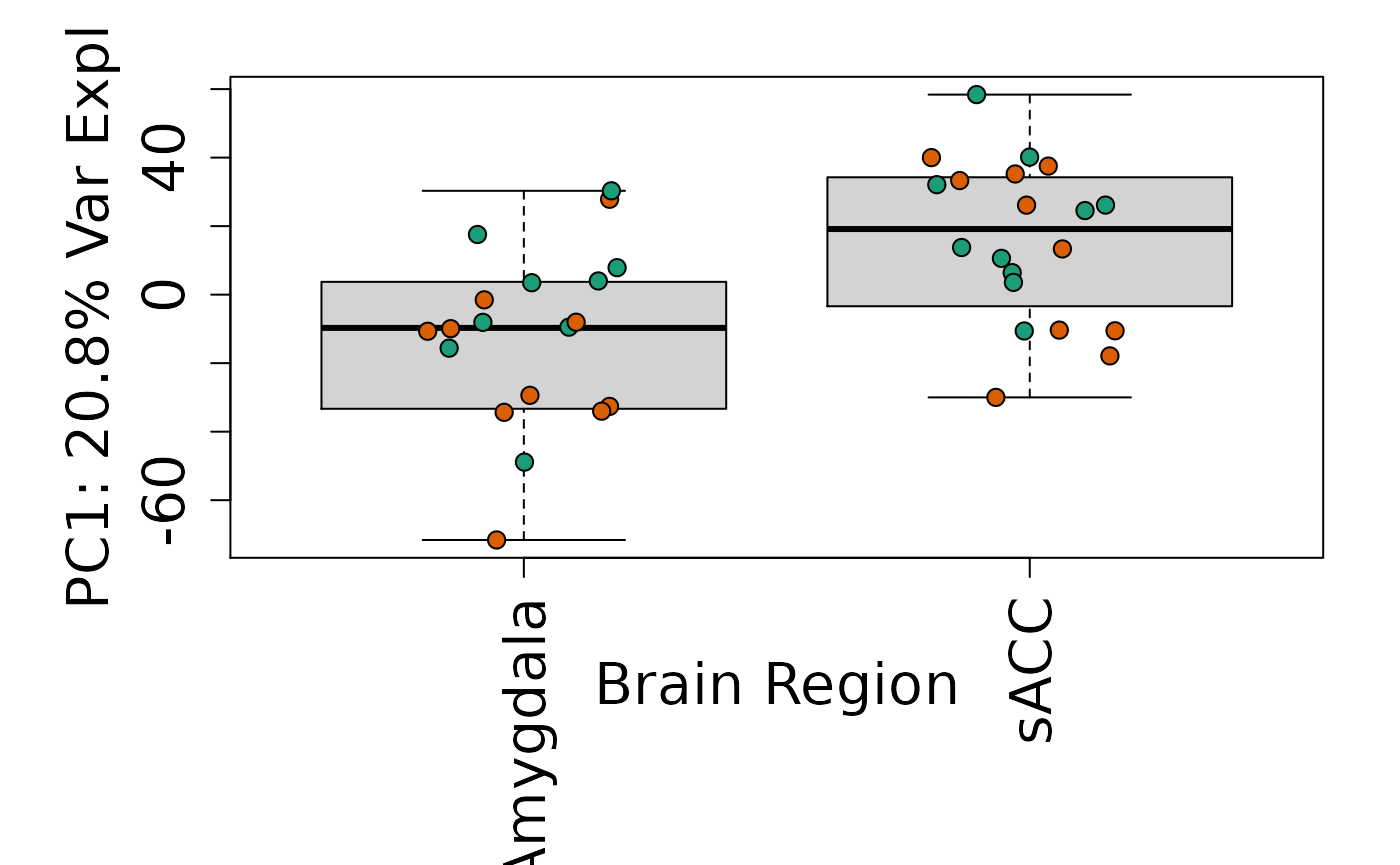
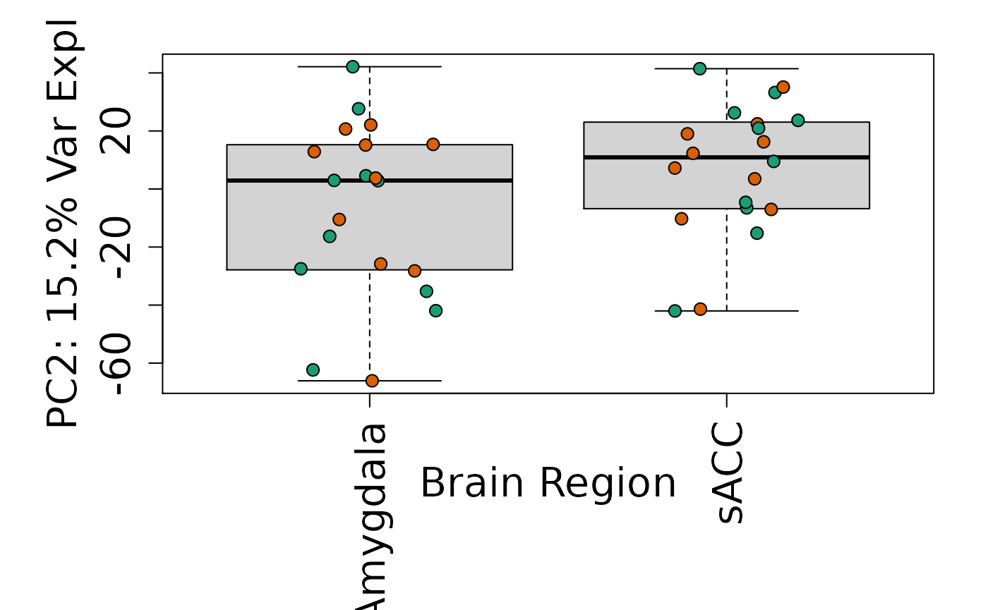
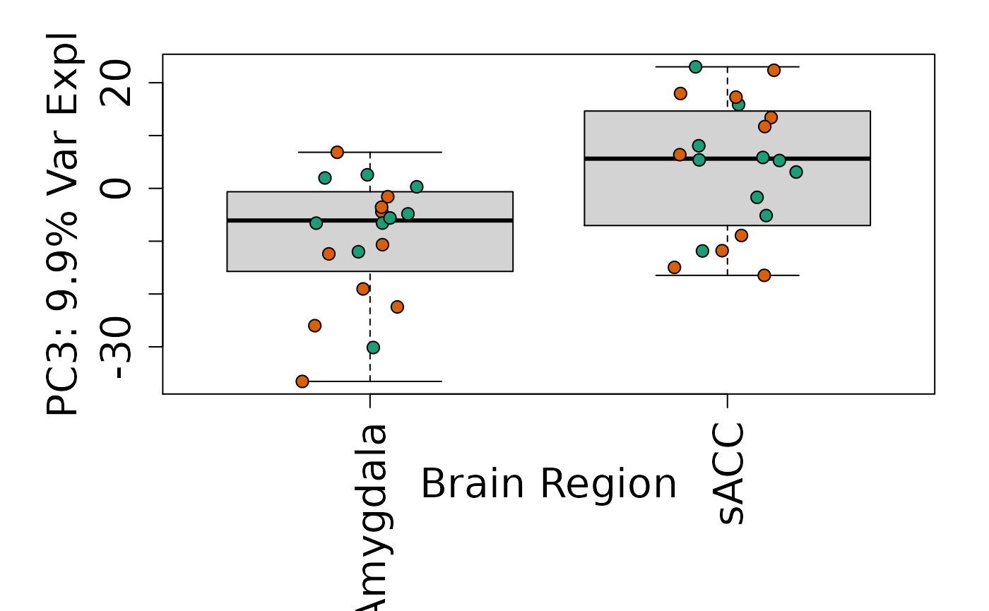
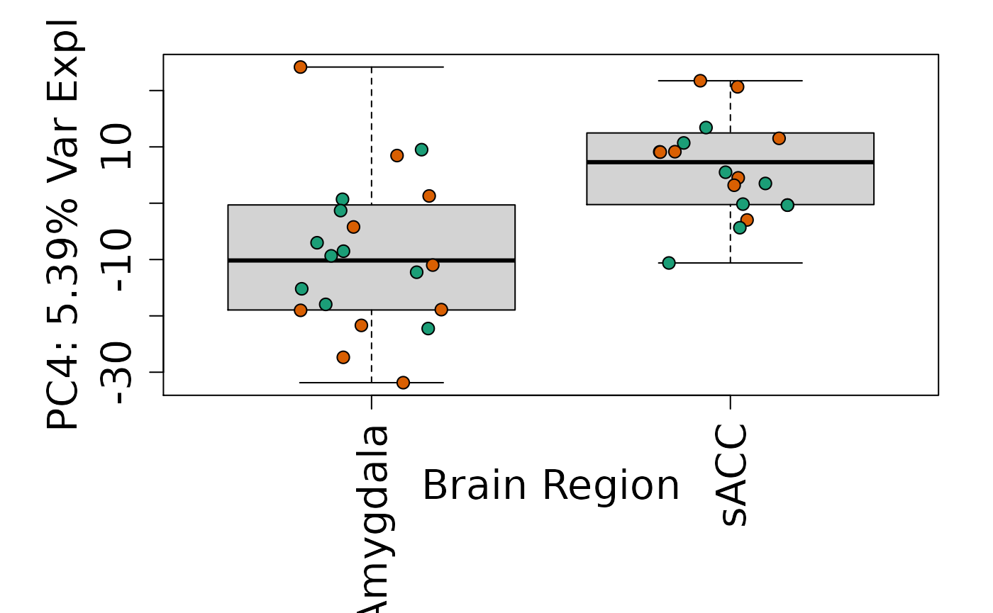
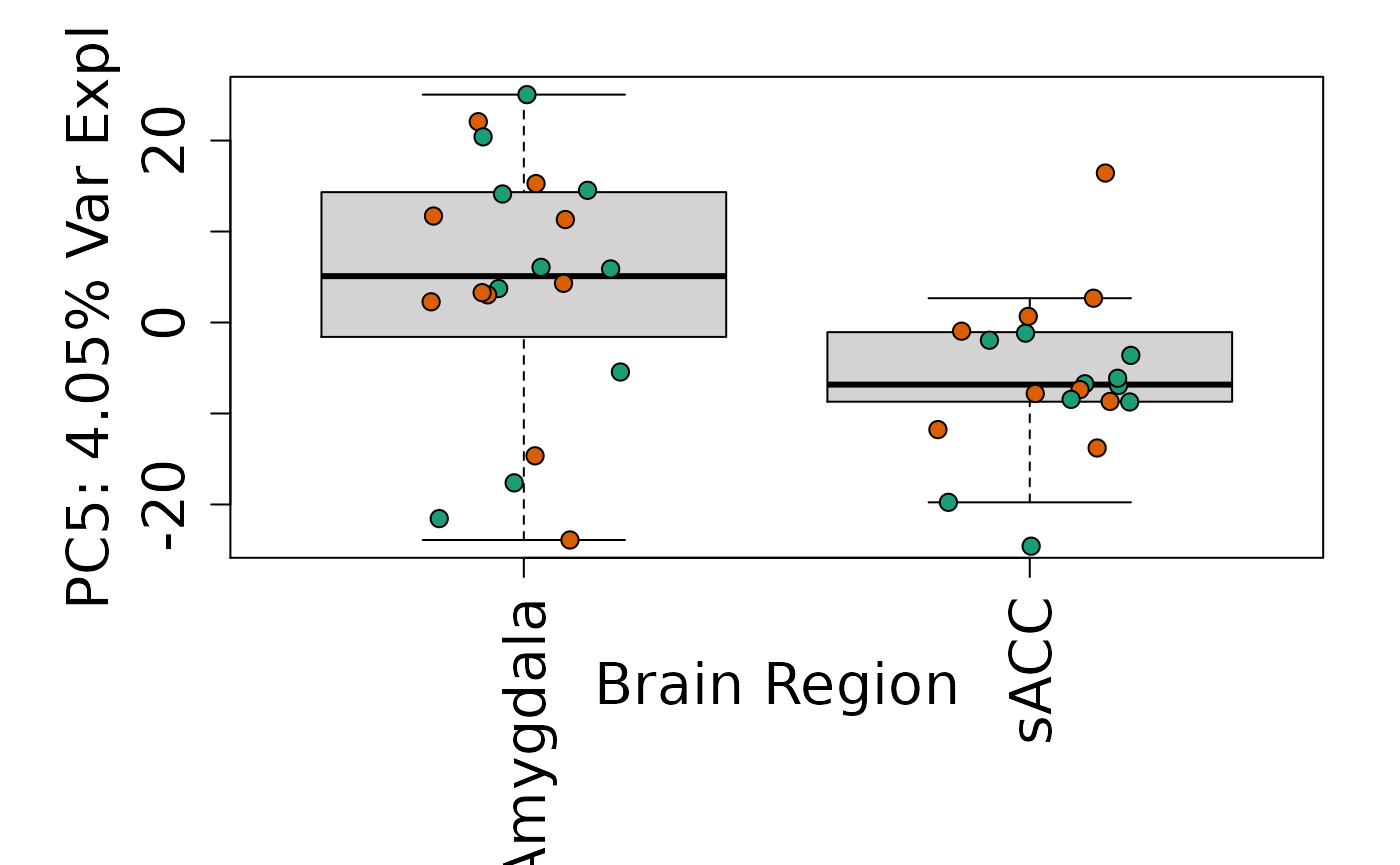
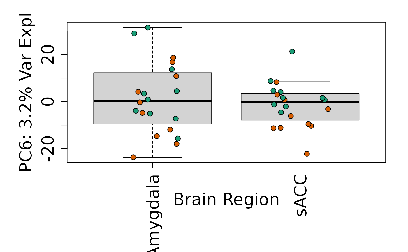
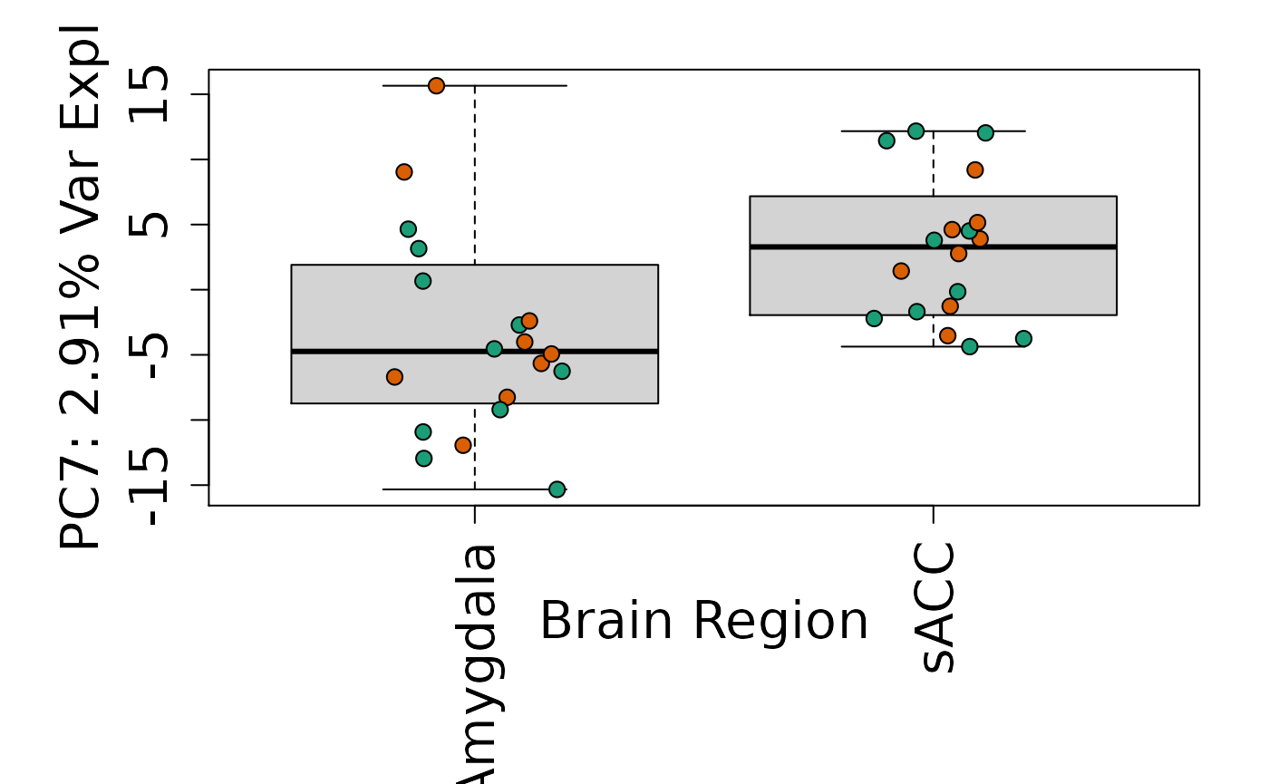
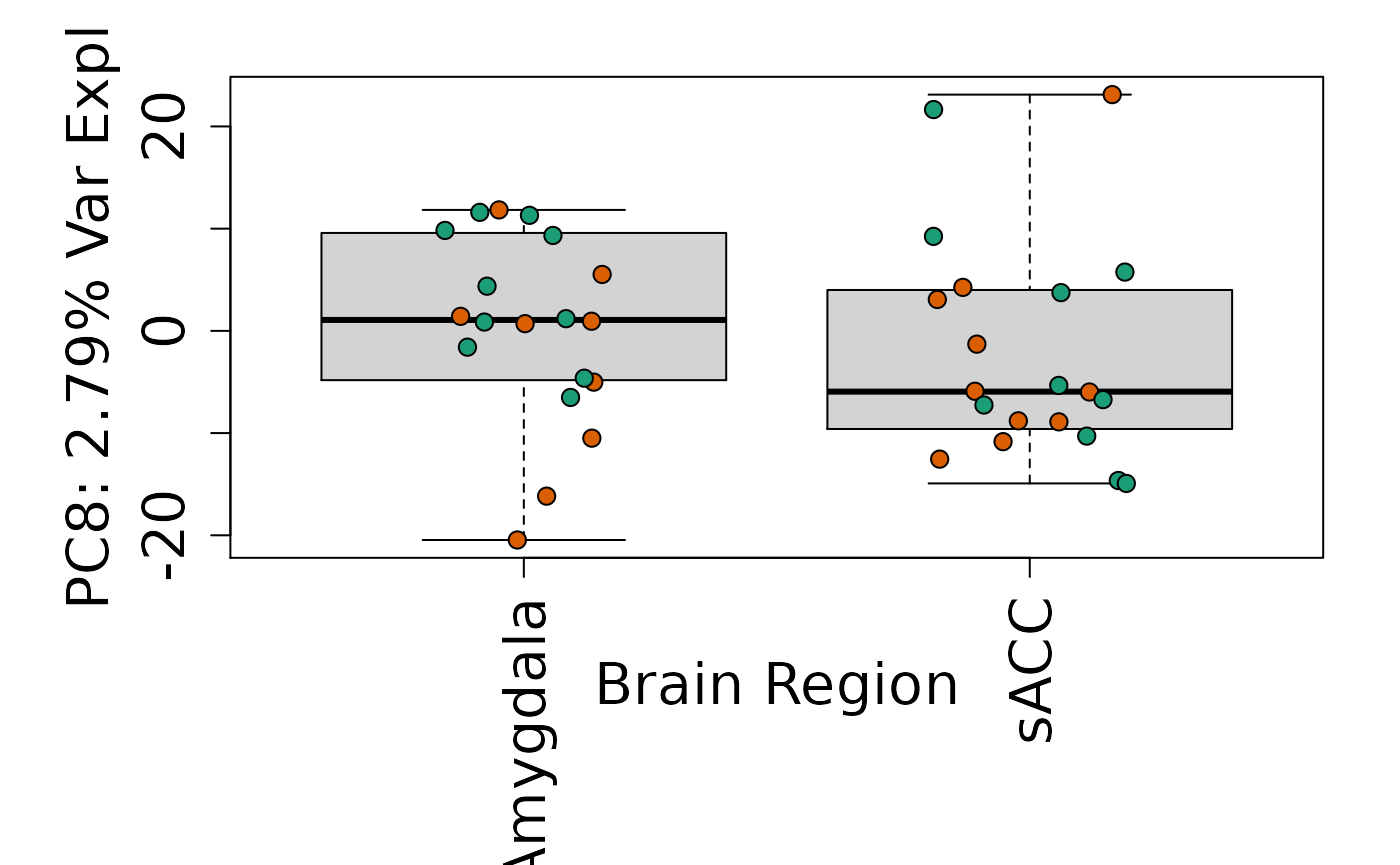
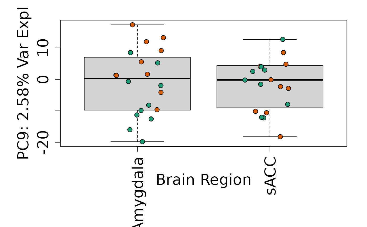
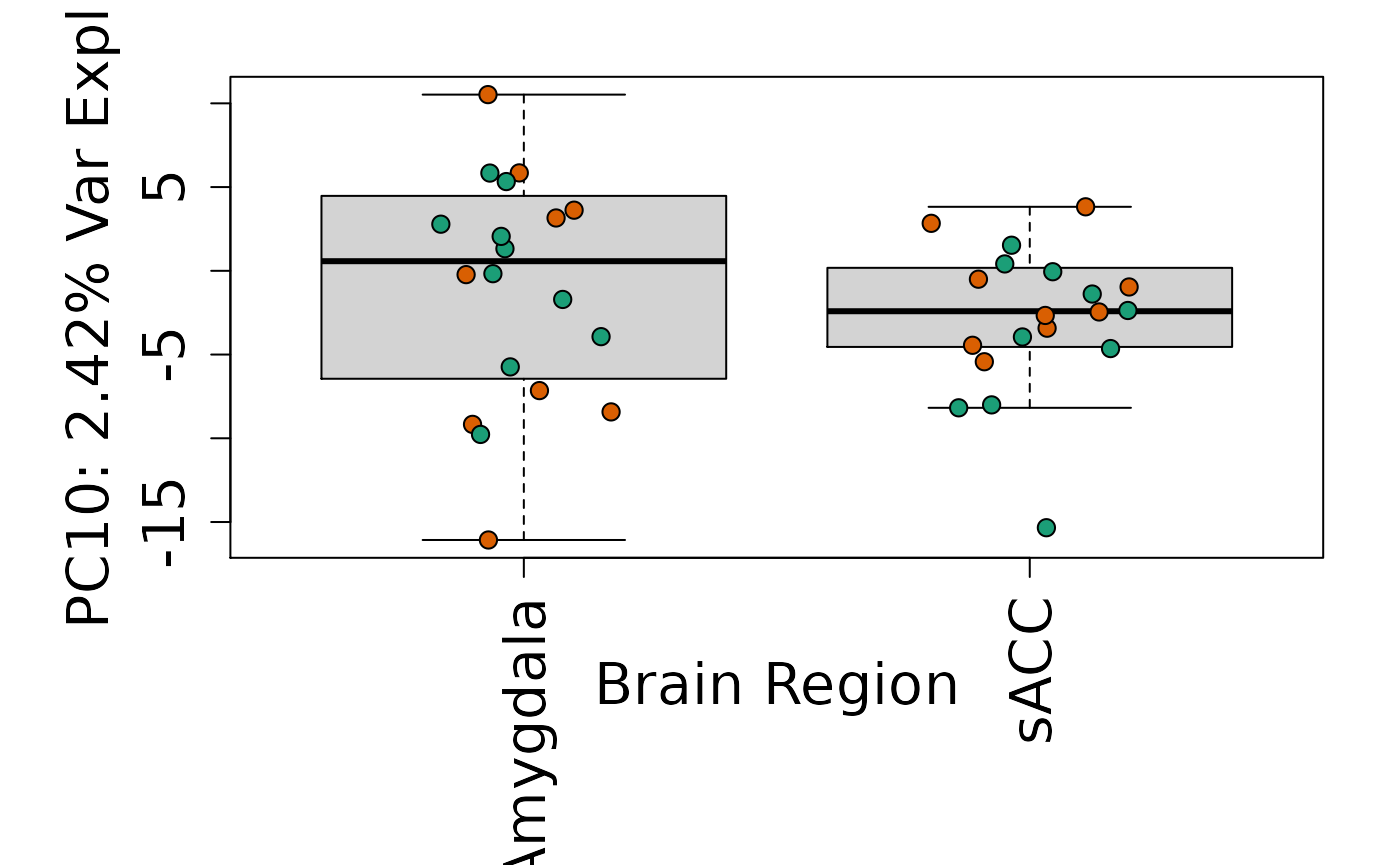
Is sex or brain region associated with any principal component from the gene expression data?
Modeling
Once we have explored our data, we can proceed to performing differential expression analyses using for example the limma package, among other Bioconductor packages. Our data exploration should inform what model we want to use. Note that in our data we have repeated measures from the same donor brains (BrNum) which we can adjust using the function duplicateCorrelation().
dge <- DGEList(
    counts = assays(rse_gene)$counts,
    genes = rowData(rse_gene)
)
dge <- calcNormFactors(dge)

# Define a model of interest (feel free to play around with other models)
mod <- model.matrix(~ PrimaryDx + PC + BrainRegion,
    data = colData(rse_gene)
)

# Mean-variance
vGene <- voom(dge, mod, plot = TRUE)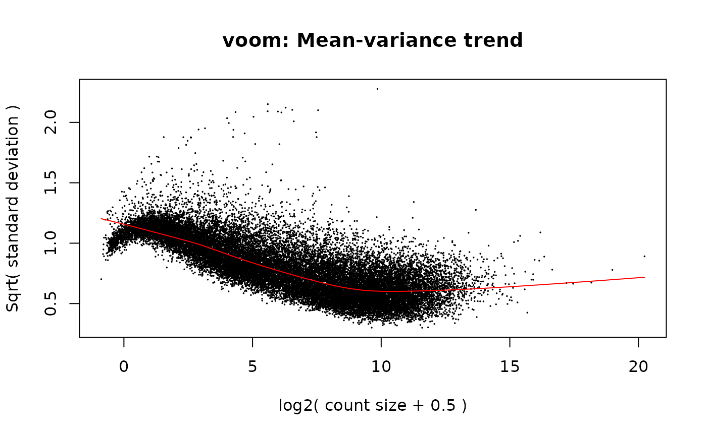
# Get duplicate correlation
gene_dupCorr <- duplicateCorrelation(vGene$E, mod,
    block = colData(rse_gene)$BrNum
)
gene_dupCorr$consensus.correlation
#> [1] 0.5626941

## We can save this for later since it can take a while
## to compute and we might need it. This will be useful
## for larger projects.
# save(gene_dupCorr,
#     file = here("DE_analysis", "rdas", "gene_dupCorr_neurons.rda")
# )

# Fit linear model
fitGeneDupl <- lmFit(
    vGene,
    correlation = gene_dupCorr$consensus.correlation,
    block = colData(rse_gene)$BrNum
)

# Here we perform an empirical Bayesian calculation to obtain our significant genes
ebGeneDupl <- eBayes(fitGeneDupl)
outGeneDupl <- topTable(
    ebGeneDupl,
    coef = 2,
    p.value = 1,
    number = nrow(rse_gene),
    sort.by = "none"
)

# Explore the distribution of differential expression p-values
hist(outGeneDupl$P.Value)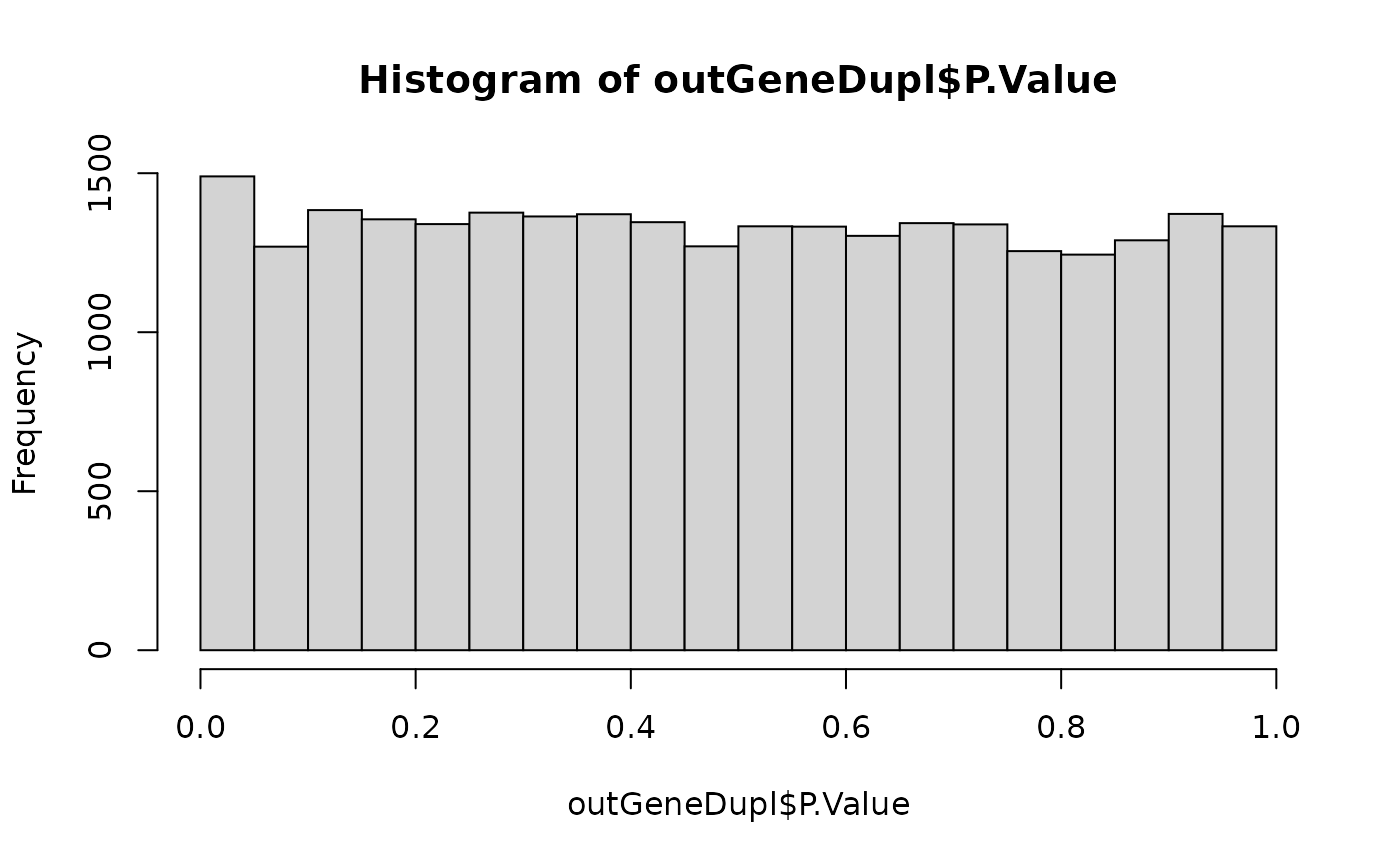
## Check how many of the genes are FDR < 5% and 10%
table(outGeneDupl$adj.P.Val < 0.05)
#>
#> FALSE
#> 26708
table(outGeneDupl$adj.P.Val < 0.1)
#>
#> FALSE TRUE
#> 26707 1
## Keep those genes iwth a p-value < 0.2
sigGeneDupl <- topTable(
ebGeneDupl,
coef = 2,
p.value = 0.2,
number = nrow(rse_gene)
)
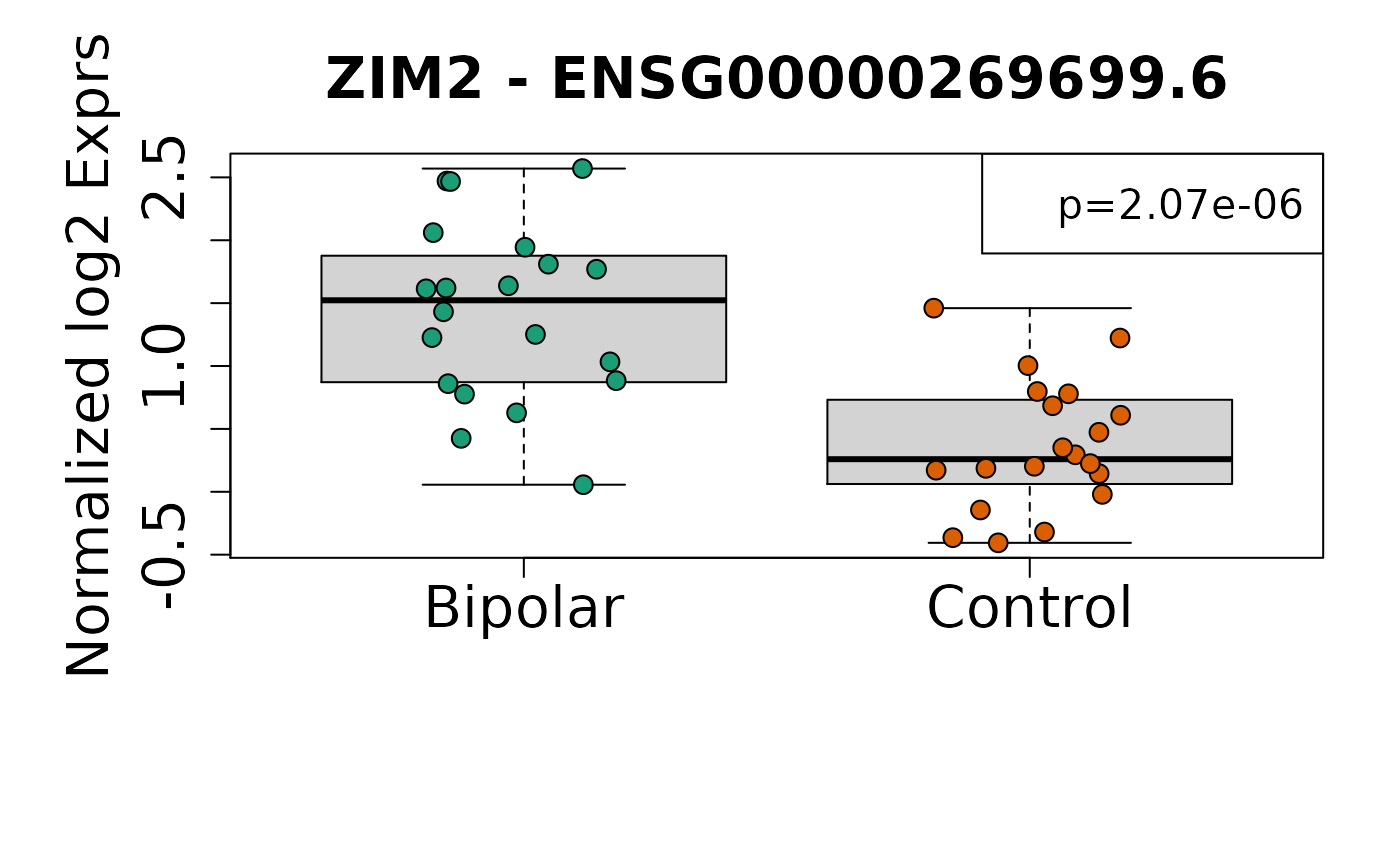
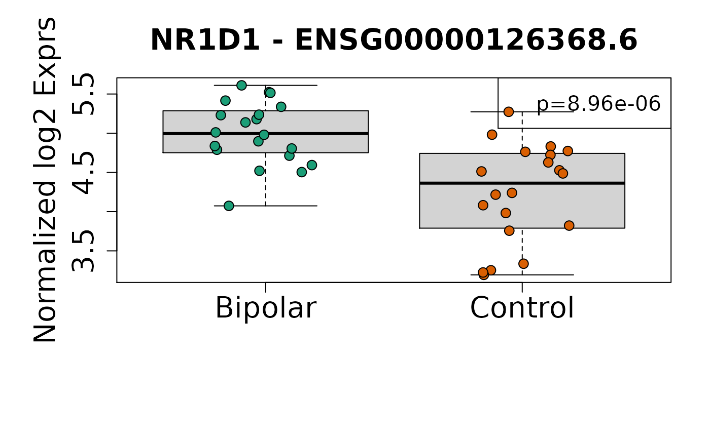
sigGeneDupl[, c("Symbol", "logFC", "P.Value", "AveExpr")]
#> Symbol logFC P.Value AveExpr
#> ENSG00000269699.6 ZIM2 -1.0860109 2.073084e-06 0.8970203
#> ENSG00000126368.6 NR1D1 -0.7676477 8.956110e-06 4.6128957
sigGeneDupl[sigGeneDupl$logFC > 0, c("Symbol", "logFC", "P.Value")]
#> [1] Symbol logFC P.Value
#> <0 rows> (or 0-length row.names)
sigGeneDupl[sigGeneDupl$logFC < 0, c("Symbol", "logFC", "P.Value")]
#> Symbol logFC P.Value
#> ENSG00000269699.6 ZIM2 -1.0860109 2.073084e-06
#> ENSG00000126368.6 NR1D1 -0.7676477 8.956110e-06
# write.csv(outGeneDupl,
# file = here("DE_analysis", "tables", "de_stats_allExprs.csv")
# )
# write.csv(sigGeneDupl,
# file = here("DE_analysis", "tables", "de_stats_fdr20_sorted.csv")
# )Check plots
Once you have identified candidate differentially expressed genes, it can be useful to visualize their expression values. Here we visualize the expression for the top two genes using boxplots.
exprs <- vGene$E[rownames(sigGeneDupl), ]

# Group together code for displaying boxplots
set.seed(20201006)
par(
    mar = c(8, 6, 4, 2),
    cex.axis = 1.8,
    cex.lab = 1.8,
    cex.main = 1.8
)
palette(brewer.pal(4, "Dark2"))

for (i in 1:nrow(sigGeneDupl)) {
    yy <- exprs[i, ]
    boxplot(
        yy ~ rse_gene$PrimaryDx,
        outline = FALSE,
        ylim = range(yy),
        ylab = "Normalized log2 Exprs",
        xlab = "",
        main = paste(sigGeneDupl$Symbol[i], "-", sigGeneDupl$gencodeID[i])
    )
    points(
        yy ~ jitter(as.numeric(rse_gene$PrimaryDx)),
        pch = 21,
        bg = rse_gene$PrimaryDx,
        cex = 1.3
    )
    ll <-
        ifelse(sigGeneDupl$logFC[i] > 0, "topleft", "topright")
    legend(ll, paste0("p=", signif(sigGeneDupl$P.Value[i], 3)), cex = 1.3)
}
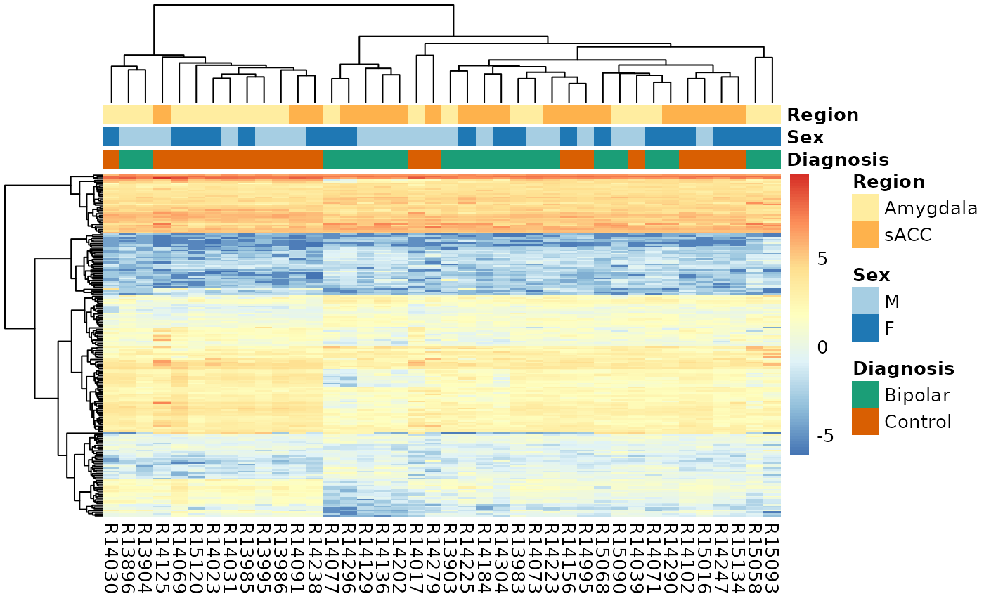
Visualize differentially expressed genes
Here we visualize differentially expressed genes (DEGs) with a heatmap.
# Get significant genes by sign
sigGene <- outGeneDupl[outGeneDupl$P.Value < 0.005, ]

exprs_heatmap <- vGene$E[rownames(sigGene), ]

df <-
    as.data.frame(colData(rse_gene)[, c("PrimaryDx", "Sex", "BrainRegion")])
rownames(df) <-
    colnames(exprs_heatmap) <- gsub("_.*", "", colnames(exprs_heatmap))
colnames(df) <- c("Diagnosis", "Sex", "Region")

#  Manually determine coloring for plot annotation
palette_names <- c("Dark2", "Paired", "YlOrRd")
ann_colors <- list()
for (i in 1:ncol(df)) {
    col_name <- colnames(df)[i]
    n_uniq_colors <- length(unique(df[, col_name]))

    #   Use a unique palette with the correct number of levels, named with
    #   those levels
    ann_colors[[col_name]] <-
        brewer.pal(n_uniq_colors, palette_names[i])[seq_len(n_uniq_colors)]
    names(ann_colors[[col_name]]) <- unique(df[, col_name])
}
#> Warning in brewer.pal(n_uniq_colors, palette_names[i]): minimal value for n is 3, returning requested palette with 3 different levels

#> Warning in brewer.pal(n_uniq_colors, palette_names[i]): minimal value for n is 3, returning requested palette with 3 different levels

#> Warning in brewer.pal(n_uniq_colors, palette_names[i]): minimal value for n is 3, returning requested palette with 3 different levels

# Display heatmap
pheatmap(
    exprs_heatmap,
    cluster_rows = TRUE,
    show_rownames = FALSE,
    cluster_cols = TRUE,
    annotation_col = df,
    annotation_colors = ann_colors
)
Gene ontology
We will use clusterProfiler to check if the differentially expressed genes are enriched in certain gene ontology terms and KEGG pathways. Running this code takes a a couple of minutes, so please be patient.
sigGeneList <-
    split(as.character(sigGene$EntrezID), sign(sigGene$logFC))
sigGeneList <- lapply(sigGeneList, function(x) {
      x[!is.na(x)]
  })
geneUniverse <- as.character(outGeneDupl$EntrezID)
geneUniverse <- geneUniverse[!is.na(geneUniverse)]

# Do GO and KEGG
goBP_Adj <- compareCluster(
    sigGeneList,
    fun = "enrichGO",
    universe = geneUniverse,
    OrgDb = org.Hs.eg.db,
    ont = "BP",
    pAdjustMethod = "BH",
    pvalueCutoff = 1,
    qvalueCutoff = 1,
    readable = TRUE
)

goMF_Adj <- compareCluster(
    sigGeneList,
    fun = "enrichGO",
    universe = geneUniverse,
    OrgDb = org.Hs.eg.db,
    ont = "MF",
    pAdjustMethod = "BH",
    pvalueCutoff = 1,
    qvalueCutoff = 1,
    readable = TRUE
)

goCC_Adj <- compareCluster(
    sigGeneList,
    fun = "enrichGO",
    universe = geneUniverse,
    OrgDb = org.Hs.eg.db,
    ont = "CC",
    pAdjustMethod = "BH",
    pvalueCutoff = 1,
    qvalueCutoff = 1,
    readable = TRUE
)

kegg_Adj <- compareCluster(
    sigGeneList,
    fun = "enrichKEGG",
    universe = geneUniverse,
    pAdjustMethod = "BH",
    pvalueCutoff = 1,
    qvalueCutoff = 1
)

# save(
#     goBP_Adj,
#     goCC_Adj,
#     goMF_Adj,
#     kegg_Adj,
#     file = here("DE_analysis", "rdas", "gene_set_objects_p005.rda")
# )

goList <-
    list(
        BP = goBP_Adj,
        MF = goMF_Adj,
        CC = goCC_Adj,
        KEGG = kegg_Adj
    )
goDf <-
    dplyr::bind_rows(lapply(goList, as.data.frame), .id = "Ontology")
goDf <- goDf[order(goDf$pvalue), ]

# write.csv(
#     goDf,
#     file = here("DE_analysis", "tables", "geneSet_output.csv"),
#     row.names = FALSE
# )

options(width = 130)
head(goDf[goDf$p.adjust < 0.05, c(1:5, 7)], n = 20)
#>      Ontology Cluster         ID                                           Description GeneRatio       pvalue
#> 696        BP       1 GO:0032611                         interleukin-1 beta production      6/73 2.152775e-06
#> 697        BP       1 GO:0050865                         regulation of cell activation     12/73 2.709506e-06
#> 698        BP       1 GO:0032612                              interleukin-1 production      6/73 3.747905e-06
#> 699        BP       1 GO:0002694                    regulation of leukocyte activation     11/73 7.875320e-06
#> 700        BP       1 GO:0002521                             leukocyte differentiation     11/73 8.260455e-06
#> 701        BP       1 GO:1903977           positive regulation of glial cell migration      3/73 1.751400e-05
#> 702        BP       1 GO:0032651           regulation of interleukin-1 beta production      5/73 2.175911e-05
#> 703        BP       1 GO:0002687            positive regulation of leukocyte migration      6/73 2.728969e-05
#> 704        BP       1 GO:0032652                regulation of interleukin-1 production      5/73 3.392997e-05
#> 2505       MF       1 GO:0046935    1-phosphatidylinositol-3-kinase regulator activity      3/78 3.586132e-05
#> 2403       MF      -1 GO:0070888                                         E-box binding      3/27 5.240514e-05
#> 705        BP       1 GO:0042116                                 macrophage activation      5/73 5.417072e-05
#> 706        BP       1 GO:1903975                    regulation of glial cell migration      3/73 6.513291e-05
#> 707        BP       1 GO:0009617                                 response to bacterium     10/73 6.787695e-05
#> 708        BP       1 GO:0050867                positive regulation of cell activation      8/73 7.145608e-05
#> 709        BP       1 GO:0060216                                definitive hemopoiesis      3/73 7.985372e-05
#> 2506       MF       1 GO:0035014      phosphatidylinositol 3-kinase regulator activity      3/78 8.982040e-05
#> 710        BP       1 GO:0071346                 cellular response to interferon-gamma      6/73 9.340196e-05
#> 711        BP       1 GO:0032640                      tumor necrosis factor production      5/73 1.034823e-04
#> 712        BP       1 GO:0071706 tumor necrosis factor superfamily cytokine production      5/73 1.152814e-04
For some examples on how to visualize the gene ontology results, check our longer guide in SPEAQeasy-example.
Acknowledgements
Members of the (former) Jaffe Lab
- Emily Burke: much of the code for SPEAQeasy before it was re-built with Nextflow, including a great portion of the R scripts still used now
- Brianna Barry: guidance, naming, and testing SPEAQeasy, leading to features such as per-sample logs and automatic strand inference, among others
- Louise Huuki: help with our guide involving resolving sample swaps from SPEAQeasy outputs
- BaDoi Phan: development of the pipeline before using Nextflow
- Andrew Jaffe: principal investigator, leading and overseeing the SPEAQeasy project
- Leonardo Collado Torres: development, guidance, and help throughout the SPEAQeasy project; development of this workshop package and website
Reproducibility
The SPEAQeasyWorkshop2020 package (Eagles, Stolz, and Collado-Torres, 2020) was made possible thanks to:
- R (R Core Team, 2020)
- BiocStyle (Oleś, Morgan, and Huber, 2020)
- clusterProfiler (Yu, Wang, Han, and He, 2012)
- dplyr (Wickham, François, Henry, and Müller, 2020)
- edgeR
- here (Müller, 2020)
- jaffelab (Collado-Torres, Jaffe, and Burke, 2019)
- limma (Ritchie, Phipson, Wu, Hu, Law, Shi, and Smyth, 2015)
- knitr (Xie, 2020)
- org.Hs.eg.db (Carlson, 2020)
- pheatmap (Kolde, 2019)
- RColorBrewer (Neuwirth, 2014)
- recount
- RefManageR (McLean, 2017)
- rmarkdown (Allaire, Xie, McPherson, Luraschi, Ushey, Atkins, Wickham, Cheng, Chang, and Iannone, 2020)
- sessioninfo (Csárdi, core, Wickham, Chang, Flight, Müller, and Hester, 2018)
- SummarizedExperiment (Morgan, Obenchain, Hester, and Pagès, 2020)
- tidyr (Wickham, 2020)
- VariantAnnotation (Obenchain, Lawrence, Carey, Gogarten, Shannon, and Morgan, 2014)
- voom (Law, Chen, Shi, and Smyth, 2014)
This package was developed using biocthis.
Code for creating the vignette
## Create the vignette
library("rmarkdown")
system.time(render("SPEAQeasyWorkshop2020.Rmd", "BiocStyle::html_document"))

## Extract the R code
library("knitr")
knit("SPEAQeasyWorkshop2020.Rmd", tangle = TRUE)
Date the vignette was generated.
#> [1] "2020-12-16 02:17:00 UTC"Wallclock time spent generating the vignette.
#> Time difference of 3.397 minsR session information.
#> ─ Session info ───────────────────────────────────────────────────────────────────────────────────────────────────────
#>  setting  value
#>  version  R version 4.0.3 (2020-10-10)
#>  os       Ubuntu 20.04 LTS
#>  system   x86_64, linux-gnu
#>  ui       X11
#>  language (EN)
#>  collate  en_US.UTF-8
#>  ctype    en_US.UTF-8
#>  tz       Etc/UTC
#>  date     2020-12-16
#>
#> ─ Packages ───────────────────────────────────────────────────────────────────────────────────────────────────────────
#>  package              * version  date       lib source
#>  AnnotationDbi        * 1.52.0   2020-10-27 [1] Bioconductor
#>  askpass                1.1      2019-01-13 [2] RSPM (R 4.0.0)
#>  assertthat             0.2.1    2019-03-21 [2] RSPM (R 4.0.0)
#>  backports              1.2.1    2020-12-09 [1] RSPM (R 4.0.3)
#>  base64enc              0.1-3    2015-07-28 [2] RSPM (R 4.0.0)
#>  Biobase              * 2.50.0   2020-10-27 [1] Bioconductor
#>  BiocFileCache          1.14.0   2020-10-27 [1] Bioconductor
#>  BiocGenerics         * 0.36.0   2020-10-27 [1] Bioconductor
#>  BiocManager            1.30.10  2019-11-16 [2] CRAN (R 4.0.3)
#>  BiocParallel           1.24.1   2020-11-06 [1] Bioconductor
#>  BiocStyle            * 2.18.1   2020-11-24 [1] Bioconductor
#>  biomaRt                2.46.0   2020-10-27 [1] Bioconductor
#>  Biostrings           * 2.58.0   2020-10-27 [1] Bioconductor
#>  bit                    4.0.4    2020-08-04 [1] RSPM (R 4.0.2)
#>  bit64                  4.0.5    2020-08-30 [1] RSPM (R 4.0.2)
#>  bitops                 1.0-6    2013-08-17 [1] RSPM (R 4.0.0)
#>  blob                   1.2.1    2020-01-20 [1] RSPM (R 4.0.0)
#>  bookdown               0.21     2020-10-13 [1] RSPM (R 4.0.2)
#>  BSgenome               1.58.0   2020-10-27 [1] Bioconductor
#>  bumphunter             1.32.0   2020-10-27 [1] Bioconductor
#>  checkmate              2.0.0    2020-02-06 [1] RSPM (R 4.0.0)
#>  cli                    2.2.0    2020-11-20 [2] RSPM (R 4.0.3)
#>  cluster                2.1.0    2019-06-19 [3] CRAN (R 4.0.3)
#>  clusterProfiler      * 3.18.0   2020-10-27 [1] Bioconductor
#>  codetools              0.2-18   2020-11-04 [3] RSPM (R 4.0.3)
#>  colorspace             2.0-0    2020-11-11 [1] RSPM (R 4.0.3)
#>  cowplot                1.1.0    2020-09-08 [1] RSPM (R 4.0.2)
#>  crayon                 1.3.4    2017-09-16 [2] RSPM (R 4.0.0)
#>  curl                   4.3      2019-12-02 [2] RSPM (R 4.0.0)
#>  data.table             1.13.4   2020-12-08 [1] RSPM (R 4.0.3)
#>  DBI                    1.1.0    2019-12-15 [1] RSPM (R 4.0.0)
#>  dbplyr                 2.0.0    2020-11-03 [1] RSPM (R 4.0.3)
#>  DelayedArray           0.16.0   2020-10-27 [1] Bioconductor
#>  derfinder              1.24.0   2020-10-27 [1] Bioconductor
#>  derfinderHelper        1.24.0   2020-10-27 [1] Bioconductor
#>  desc                   1.2.0    2018-05-01 [2] RSPM (R 4.0.0)
#>  digest                 0.6.27   2020-10-24 [2] RSPM (R 4.0.3)
#>  DO.db                  2.9      2020-11-25 [1] Bioconductor
#>  doRNG                  1.8.2    2020-01-27 [1] RSPM (R 4.0.0)
#>  DOSE                   3.16.0   2020-10-27 [1] Bioconductor
#>  downloader             0.4      2015-07-09 [1] RSPM (R 4.0.0)
#>  dplyr                  1.0.2    2020-08-18 [1] RSPM (R 4.0.2)
#>  edgeR                * 3.32.0   2020-10-27 [1] Bioconductor
#>  ellipsis               0.3.1    2020-05-15 [2] RSPM (R 4.0.0)
#>  enrichplot             1.10.1   2020-11-14 [1] Bioconductor
#>  evaluate               0.14     2019-05-28 [2] RSPM (R 4.0.0)
#>  fansi                  0.4.1    2020-01-08 [2] RSPM (R 4.0.0)
#>  farver                 2.0.3    2020-01-16 [1] RSPM (R 4.0.0)
#>  fastmatch              1.1-0    2017-01-28 [1] RSPM (R 4.0.0)
#>  fgsea                  1.16.0   2020-10-27 [1] Bioconductor
#>  foreach                1.5.1    2020-10-15 [1] RSPM (R 4.0.2)
#>  foreign                0.8-80   2020-05-24 [3] CRAN (R 4.0.3)
#>  Formula                1.2-4    2020-10-16 [1] RSPM (R 4.0.2)
#>  fs                     1.5.0    2020-07-31 [2] RSPM (R 4.0.2)
#>  generics               0.1.0    2020-10-31 [1] RSPM (R 4.0.3)
#>  GenomeInfoDb         * 1.26.2   2020-12-08 [1] Bioconductor
#>  GenomeInfoDbData       1.2.4    2020-11-25 [1] Bioconductor
#>  GenomicAlignments      1.26.0   2020-10-27 [1] Bioconductor
#>  GenomicFeatures        1.42.1   2020-11-12 [1] Bioconductor
#>  GenomicFiles           1.26.0   2020-10-27 [1] Bioconductor
#>  GenomicRanges        * 1.42.0   2020-10-27 [1] Bioconductor
#>  GEOquery               2.58.0   2020-10-27 [1] Bioconductor
#>  ggforce                0.3.2    2020-06-23 [1] RSPM (R 4.0.2)
#>  ggplot2                3.3.2    2020-06-19 [1] RSPM (R 4.0.1)
#>  ggraph                 2.0.4    2020-11-16 [1] RSPM (R 4.0.3)
#>  ggrepel                0.8.2    2020-03-08 [1] RSPM (R 4.0.2)
#>  glue                   1.4.2    2020-08-27 [2] RSPM (R 4.0.2)
#>  GO.db                  3.12.1   2020-11-25 [1] Bioconductor
#>  googledrive            1.0.1    2020-05-05 [1] RSPM (R 4.0.0)
#>  GOSemSim               2.16.1   2020-10-29 [1] Bioconductor
#>  graphlayouts           0.7.1    2020-10-26 [1] RSPM (R 4.0.3)
#>  gridExtra              2.3      2017-09-09 [1] RSPM (R 4.0.0)
#>  gtable                 0.3.0    2019-03-25 [1] RSPM (R 4.0.0)
#>  Hmisc                  4.4-2    2020-11-29 [1] RSPM (R 4.0.3)
#>  hms                    0.5.3    2020-01-08 [1] RSPM (R 4.0.0)
#>  htmlTable              2.1.0    2020-09-16 [1] RSPM (R 4.0.2)
#>  htmltools              0.5.0    2020-06-16 [2] RSPM (R 4.0.1)
#>  htmlwidgets            1.5.3    2020-12-10 [2] RSPM (R 4.0.3)
#>  httr                   1.4.2    2020-07-20 [2] RSPM (R 4.0.2)
#>  igraph                 1.2.6    2020-10-06 [1] RSPM (R 4.0.2)
#>  IRanges              * 2.24.1   2020-12-12 [1] Bioconductor
#>  iterators              1.0.13   2020-10-15 [1] RSPM (R 4.0.2)
#>  jaffelab             * 0.99.30  2020-11-25 [1] Github (LieberInstitute/jaffelab@42637ff)
#>  jpeg                   0.1-8.1  2019-10-24 [1] RSPM (R 4.0.0)
#>  jsonlite               1.7.2    2020-12-09 [2] RSPM (R 4.0.3)
#>  knitr                  1.30     2020-09-22 [2] RSPM (R 4.0.2)
#>  lattice                0.20-41  2020-04-02 [3] CRAN (R 4.0.3)
#>  latticeExtra           0.6-29   2019-12-19 [1] RSPM (R 4.0.0)
#>  lifecycle              0.2.0    2020-03-06 [2] RSPM (R 4.0.0)
#>  limma                * 3.46.0   2020-10-27 [1] Bioconductor
#>  locfit                 1.5-9.4  2020-03-25 [1] RSPM (R 4.0.0)
#>  lubridate              1.7.9.2  2020-11-13 [1] RSPM (R 4.0.3)
#>  magrittr               2.0.1    2020-11-17 [2] RSPM (R 4.0.3)
#>  MASS                   7.3-53   2020-09-09 [3] CRAN (R 4.0.3)
#>  Matrix                 1.2-18   2019-11-27 [3] CRAN (R 4.0.3)
#>  MatrixGenerics       * 1.2.0    2020-10-27 [1] Bioconductor
#>  matrixStats          * 0.57.0   2020-09-25 [1] RSPM (R 4.0.2)
#>  memoise                1.1.0    2017-04-21 [2] RSPM (R 4.0.0)
#>  munsell                0.5.0    2018-06-12 [1] RSPM (R 4.0.0)
#>  nnet                   7.3-14   2020-04-26 [3] CRAN (R 4.0.3)
#>  openssl                1.4.3    2020-09-18 [2] RSPM (R 4.0.2)
#>  org.Hs.eg.db         * 3.12.0   2020-11-25 [1] Bioconductor
#>  pheatmap             * 1.0.12   2019-01-04 [1] RSPM (R 4.0.0)
#>  pillar                 1.4.7    2020-11-20 [2] RSPM (R 4.0.3)
#>  pkgconfig              2.0.3    2019-09-22 [2] RSPM (R 4.0.0)
#>  pkgdown                1.6.1    2020-09-12 [1] RSPM (R 4.0.2)
#>  plyr                   1.8.6    2020-03-03 [1] RSPM (R 4.0.2)
#>  png                    0.1-7    2013-12-03 [1] RSPM (R 4.0.0)
#>  polyclip               1.10-0   2019-03-14 [1] RSPM (R 4.0.0)
#>  prettyunits            1.1.1    2020-01-24 [2] RSPM (R 4.0.0)
#>  progress               1.2.2    2019-05-16 [1] RSPM (R 4.0.0)
#>  purrr                  0.3.4    2020-04-17 [2] RSPM (R 4.0.0)
#>  qvalue                 2.22.0   2020-10-27 [1] Bioconductor
#>  R6                     2.5.0    2020-10-28 [2] RSPM (R 4.0.3)
#>  rafalib              * 1.0.0    2015-08-09 [1] RSPM (R 4.0.0)
#>  ragg                   0.4.0    2020-10-05 [1] RSPM (R 4.0.3)
#>  rappdirs               0.3.1    2016-03-28 [1] RSPM (R 4.0.0)
#>  RColorBrewer         * 1.1-2    2014-12-07 [1] RSPM (R 4.0.0)
#>  Rcpp                   1.0.5    2020-07-06 [2] RSPM (R 4.0.2)
#>  RCurl                  1.98-1.2 2020-04-18 [1] RSPM (R 4.0.0)
#>  readr                  1.4.0    2020-10-05 [1] RSPM (R 4.0.3)
#>  recount              * 1.16.0   2020-10-27 [1] Bioconductor
#>  RefManageR           * 1.3.0    2020-11-25 [1] Github (ropensci/RefManageR@ab8fe60)
#>  rentrez                1.2.3    2020-11-10 [1] RSPM (R 4.0.3)
#>  reshape2               1.4.4    2020-04-09 [1] RSPM (R 4.0.2)
#>  rlang                  0.4.9    2020-11-26 [2] RSPM (R 4.0.3)
#>  rmarkdown              2.6      2020-12-14 [1] RSPM (R 4.0.3)
#>  rngtools               1.5      2020-01-23 [1] RSPM (R 4.0.0)
#>  rpart                  4.1-15   2019-04-12 [3] CRAN (R 4.0.3)
#>  rprojroot              2.0.2    2020-11-15 [2] RSPM (R 4.0.3)
#>  Rsamtools            * 2.6.0    2020-10-27 [1] Bioconductor
#>  RSQLite                2.2.1    2020-09-30 [1] RSPM (R 4.0.2)
#>  rstudioapi             0.13     2020-11-12 [2] RSPM (R 4.0.3)
#>  rtracklayer            1.50.0   2020-10-27 [1] Bioconductor
#>  rvcheck                0.1.8    2020-03-01 [1] RSPM (R 4.0.0)
#>  S4Vectors            * 0.28.1   2020-12-09 [1] Bioconductor
#>  scales                 1.1.1    2020-05-11 [1] RSPM (R 4.0.0)
#>  scatterpie             0.1.5    2020-09-09 [1] RSPM (R 4.0.2)
#>  segmented              1.3-1    2020-12-10 [1] RSPM (R 4.0.3)
#>  sessioninfo          * 1.1.1    2018-11-05 [2] RSPM (R 4.0.0)
#>  shadowtext             0.0.7    2019-11-06 [1] RSPM (R 4.0.0)
#>  statmod                1.4.35   2020-10-19 [1] RSPM (R 4.0.3)
#>  stringi                1.5.3    2020-09-09 [2] RSPM (R 4.0.2)
#>  stringr                1.4.0    2019-02-10 [2] RSPM (R 4.0.0)
#>  SummarizedExperiment * 1.20.0   2020-10-27 [1] Bioconductor
#>  survival               3.2-7    2020-09-28 [3] CRAN (R 4.0.3)
#>  systemfonts            0.3.2    2020-09-29 [1] RSPM (R 4.0.3)
#>  textshaping            0.2.1    2020-11-13 [1] RSPM (R 4.0.3)
#>  tibble                 3.0.4    2020-10-12 [2] RSPM (R 4.0.2)
#>  tidygraph              1.2.0    2020-05-12 [1] RSPM (R 4.0.2)
#>  tidyr                * 1.1.2    2020-08-27 [1] RSPM (R 4.0.3)
#>  tidyselect             1.1.0    2020-05-11 [1] RSPM (R 4.0.0)
#>  tweenr                 1.0.1    2018-12-14 [1] RSPM (R 4.0.2)
#>  VariantAnnotation    * 1.36.0   2020-10-27 [1] Bioconductor
#>  vctrs                  0.3.5    2020-11-17 [2] RSPM (R 4.0.3)
#>  viridis                0.5.1    2018-03-29 [1] RSPM (R 4.0.0)
#>  viridisLite            0.3.0    2018-02-01 [1] RSPM (R 4.0.0)
#>  withr                  2.3.0    2020-09-22 [2] RSPM (R 4.0.2)
#>  xfun                   0.19     2020-10-30 [2] RSPM (R 4.0.3)
#>  XML                    3.99-0.5 2020-07-23 [1] RSPM (R 4.0.2)
#>  xml2                   1.3.2    2020-04-23 [2] RSPM (R 4.0.0)
#>  XVector              * 0.30.0   2020-10-27 [1] Bioconductor
#>  yaml                   2.2.1    2020-02-01 [2] RSPM (R 4.0.0)
#>  zlibbioc               1.36.0   2020-10-27 [1] Bioconductor
#>
#> [1] /__w/_temp/Library
#> [2] /usr/local/lib/R/site-library
#> [3] /usr/local/lib/R/library
Bibliography
This vignette was generated using BiocStyle (Oleś, Morgan, and Huber, 2020) with knitr (Xie, 2020) and rmarkdown (Allaire, Xie, McPherson, et al., 2020) running behind the scenes.
Citations made with RefManageR (McLean, 2017).
[1] J. Allaire, Y. Xie, J. McPherson, et al. rmarkdown: Dynamic Documents for R. R package version 2.6. 2020. URL: https://github.com/rstudio/rmarkdown.
[2] M. Carlson. org.Hs.eg.db: Genome wide annotation for Human. R package version 3.12.0. 2020.
[3] L. Collado-Torres, A. E. Jaffe, and E. E. Burke. jaffelab: Commonly used functions by the Jaffe lab. R package version 0.99.30. 2019. URL: https://github.com/LieberInstitute/jaffelab.
[4] G. Csárdi, R. core, H. Wickham, et al. sessioninfo: R Session Information. R package version 1.1.1. 2018. URL: https://github.com/r-lib/sessioninfo#readme.
[5] N. J. Eagles, E. E. Burke, J. Leonard, et al. “SPEAQeasy: a Scalable Pipeline for Expression Analysis and Quantification for R/Bioconductor-powered RNA-seq analyses”. In: bioRxiv (2020). DOI: 10.1101/2020.12.11.386789. URL: https://www.biorxiv.org/content/10.1101/2020.12.11.386789v1.
[6] N. J. Eagles, J. M. Stolz, and L. Collado-Torres. EuroBioc2020 SPEAQeasy workshop. https://github.com/LieberInstitute/SPEAQeasyWorkshop2020 - R package version 0.99.0. 2020. DOI: 10.18129/B9.bioc.SPEAQeasyWorkshop2020. URL: http://www.bioconductor.org/packages/SPEAQeasyWorkshop2020.
[7] R. Kolde. pheatmap: Pretty Heatmaps. R package version 1.0.12. 2019.
[8] C. Law, Y. Chen, W. Shi, et al. “Voom: precision weights unlock linear model analysis tools for RNA-seq read counts”. In: Genome Biology 15 (2014), p. R29.
[9] M. W. McLean. “RefManageR: Import and Manage BibTeX and BibLaTeX References in R”. In: The Journal of Open Source Software (2017). DOI: 10.21105/joss.00338.
[10] M. Morgan, V. Obenchain, J. Hester, et al. SummarizedExperiment: SummarizedExperiment container. R package version 1.20.0. 2020. URL: https://bioconductor.org/packages/SummarizedExperiment.
[11] K. Müller. here: A Simpler Way to Find Your Files. https://here.r-lib.org/, https://github.com/r-lib/here. 2020.
[12] E. Neuwirth. RColorBrewer: ColorBrewer Palettes. R package version 1.1-2. 2014.
[13] V. Obenchain, M. Lawrence, V. Carey, et al. “VariantAnnotation: a Bioconductor package for exploration and annotation of genetic variants”. In: Bioinformatics 30.14 (2014), pp. 2076-2078. DOI: 10.1093/bioinformatics/btu168.
[14] A. Oleś, M. Morgan, and W. Huber. BiocStyle: Standard styles for vignettes and other Bioconductor documents. R package version 2.18.1. 2020. URL: https://github.com/Bioconductor/BiocStyle.
[15] R Core Team. R: A Language and Environment for Statistical Computing. R Foundation for Statistical Computing. Vienna, Austria, 2020. URL: https://www.R-project.org/.
[16] M. E. Ritchie, B. Phipson, D. Wu, et al. “limma powers differential expression analyses for RNA-sequencing and microarray studies”. In: Nucleic Acids Research 43.7 (2015), p. e47. DOI: 10.1093/nar/gkv007.
[17] H. Wickham. tidyr: Tidy Messy Data. https://tidyr.tidyverse.org, https://github.com/tidyverse/tidyr. 2020.
[18] H. Wickham, R. François, L. Henry, et al. dplyr: A Grammar of Data Manipulation. https://dplyr.tidyverse.org, https://github.com/tidyverse/dplyr. 2020.
[19] Y. Xie. knitr: A General-Purpose Package for Dynamic Report Generation in R. R package version 1.30. 2020. URL: https://yihui.org/knitr/.
[20] G. Yu, L. Wang, Y. Han, et al. “clusterProfiler: an R package for comparing biological themes among gene clusters”. In: OMICS: A Journal of Integrative Biology 16.5 (2012), pp. 284-287. DOI: 10.1089/omi.2011.0118.