Sample spatial gene visualization

This function visualizes the gene expression stored in assays(spe) or any continuous variable stored in colData(spe) for one given sample at the spot-level using (by default) the histology information on the background. To visualize clusters (or any discrete variable) use vis_clus().

vis_gene(
  spe,
  sampleid = unique(spe$sample_id)[1],
  geneid = rowData(spe)$gene_search[1],
  spatial = TRUE,
  assayname = "logcounts",
  minCount = 0,
  viridis = TRUE,
  image_id = "lowres",
  alpha = NA,
  cont_colors = if (viridis) viridisLite::viridis(21) else c("aquamarine4",
    "springgreen", "goldenrod", "red"),
  point_size = 2,
  auto_crop = TRUE,
  na_color = "#CCCCCC40",
  multi_gene_method = c("z_score", "pca", "sparsity"),
  is_stitched = FALSE,
  cap_percentile = 1,
  ...
)

Arguments

spe: A SpatialExperiment-class object. See fetch_data() for how to download some example objects or read10xVisiumWrapper() to read in spaceranger --count output files and build your own spe object.
sampleid: A character(1) specifying which sample to plot from colData(spe)$sample_id (formerly colData(spe)$sample_name).
geneid: A character() specifying the gene ID(s) stored in rowData(spe)$gene_search or a continuous variable(s) stored in colData(spe) to visualize. For each ID, if rowData(spe)$gene_search is missing, then rownames(spe) is used to search for the gene ID. When a vector of length > 1 is supplied, the continuous variables are combined according to multi_gene_method, producing a single value for each spot.
spatial: A logical(1) indicating whether to include the histology layer from geom_spatial(). If you plan to use ggplotly() then it's best to set this to FALSE.
assayname: The name of the assays(spe) to use for extracting the gene expression data. Defaults to logcounts.
minCount: A numeric(1) specifying the minimum gene expression (or value in the continuous variable) to visualize. Values at or below this threshold will be set to NA. Defaults to 0.
viridis: A logical(1) whether to use the color-blind friendly palette from viridis or the color palette used in the paper that was chosen for contrast when visualizing the data on top of the histology image. One issue is being able to differentiate low values from NA ones due to the purple-ish histology information that is dependent on cell density.
image_id: A character(1) with the name of the image ID you want to use in the background.
alpha: A numeric(1) in the [0, 1] range that specifies the transparency level of the data on the spots.
cont_colors: A character() vector of colors that supersedes the viridis argument.
point_size: A numeric(1) specifying the size of the points. Defaults to 1.25. Some colors look better if you use 2 for instance.
auto_crop: A logical(1) indicating whether to automatically crop the image / plotting area, which is useful if the Visium capture area is not centered on the image and if the image is not a square.
na_color: A character(1) specifying a color for the NA values. If you set alpha = NA then it's best to set na_color to a color that has alpha blending already, which will make non-NA values pop up more and the NA values will show with a lighter color. This behavior is lost when alpha is set to a non-NA value.
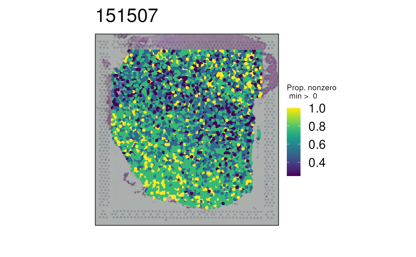
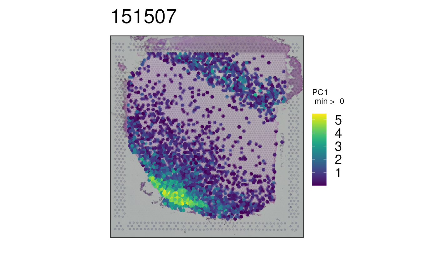
multi_gene_method: A character(1): either "pca", "sparsity", or "z_score". This parameter controls how multiple continuous variables are combined for visualization, and only applies when geneid has length great than 1. z_score: to summarize multiple continuous variables, each is normalized to represent a Z-score. The multiple scores are then averaged. pca: PCA dimension reduction is conducted on the matrix formed by the continuous variables, and the first PC is then used and multiplied by -1 if needed to have the majority of the values for PC1 to be positive. sparsity: the proportion of continuous variables with positive values for each spot is computed. For more details, check the multi gene vignette at https://research.libd.org/spatialLIBD/articles/multi_gene_plots.html.
is_stitched: A logical(1) vector: If TRUE, expects a SpatialExperiment-class built with visiumStitched::build_spe(). http://research.libd.org/visiumStitched/reference/build_spe.html; in particular, expects a logical colData column exclude_overlapping specifying which spots to exclude from the plot. Sets auto_crop = FALSE.
cap_percentile: A numeric(1) in (0, 1] determining the maximum percentile (as a proportion) at which to cap expression. For example, a value of 0.95 sets the top 5% of expression values to the 95th percentile value. This can help make the color scale more dynamic in the presence of high outliers. Defaults to 1, which effectively performs no capping.
...: Passed to paste0() for making the title of the plot following the sampleid.

Value

A ggplot2 object.

Details

This function subsets spe to the given sample and prepares the data and title for vis_gene_p(). It also adds a caption to the plot.

Examples


if (enough_ram()) {
    ## Obtain the necessary data
    if (!exists("spe")) spe <- fetch_data("spe")

    ## Valid `geneid` values are those in
    head(rowData(spe)$gene_search)
    ## or continuous variables stored in colData(spe)
    ## or rownames(spe)

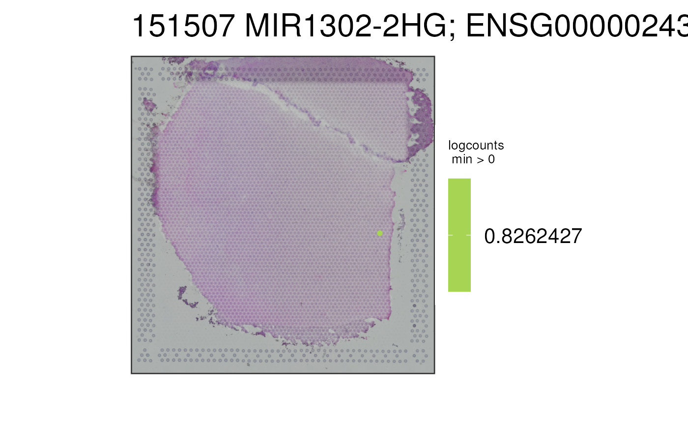
    ## Visualize a default gene on the non-viridis scale
    p1 <- vis_gene(
        spe = spe,
        sampleid = "151507",
        viridis = FALSE
    )
    print(p1)

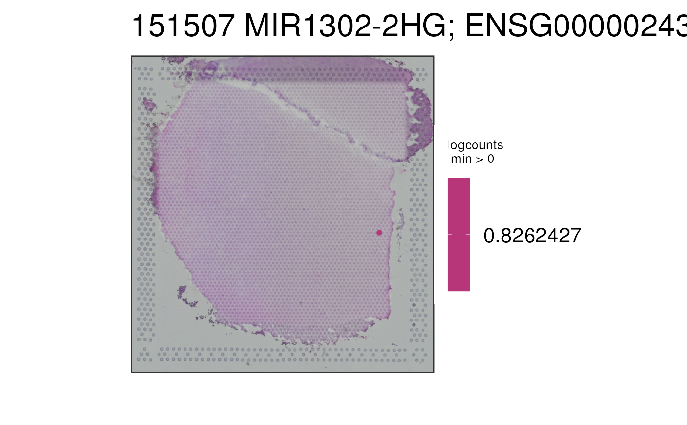
    ## Use a custom set of colors in the reverse order than usual
    p2 <- vis_gene(
        spe = spe,
        sampleid = "151507",
        cont_colors = rev(viridisLite::viridis(21, option = "magma"))
    )
    print(p2)

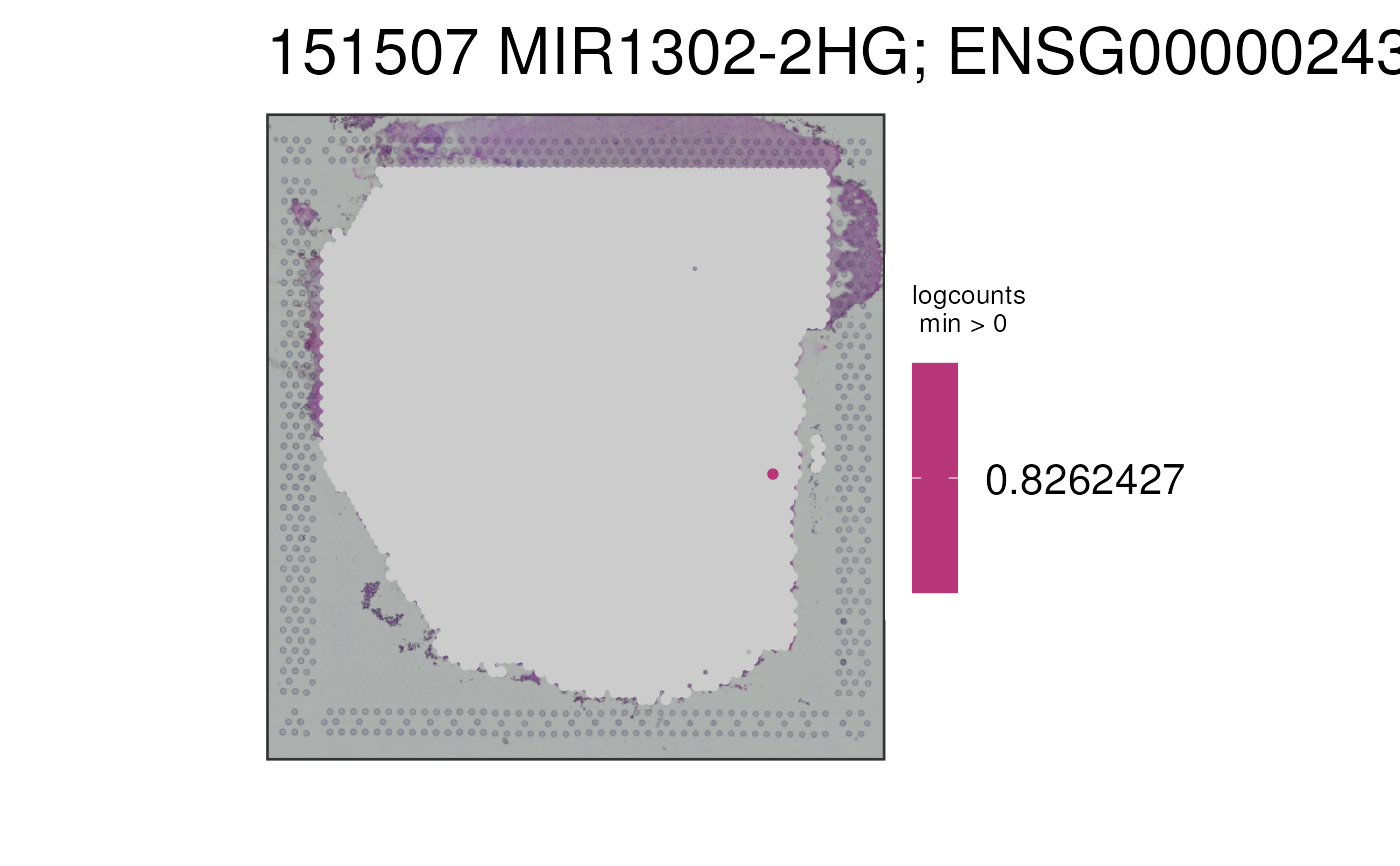
    ## Turn the alpha to 1, which makes the NA values have a full alpha
    p2b <- vis_gene(
        spe = spe,
        sampleid = "151507",
        cont_colors = rev(viridisLite::viridis(21, option = "magma")),
        alpha = 1
    )
    print(p2b)

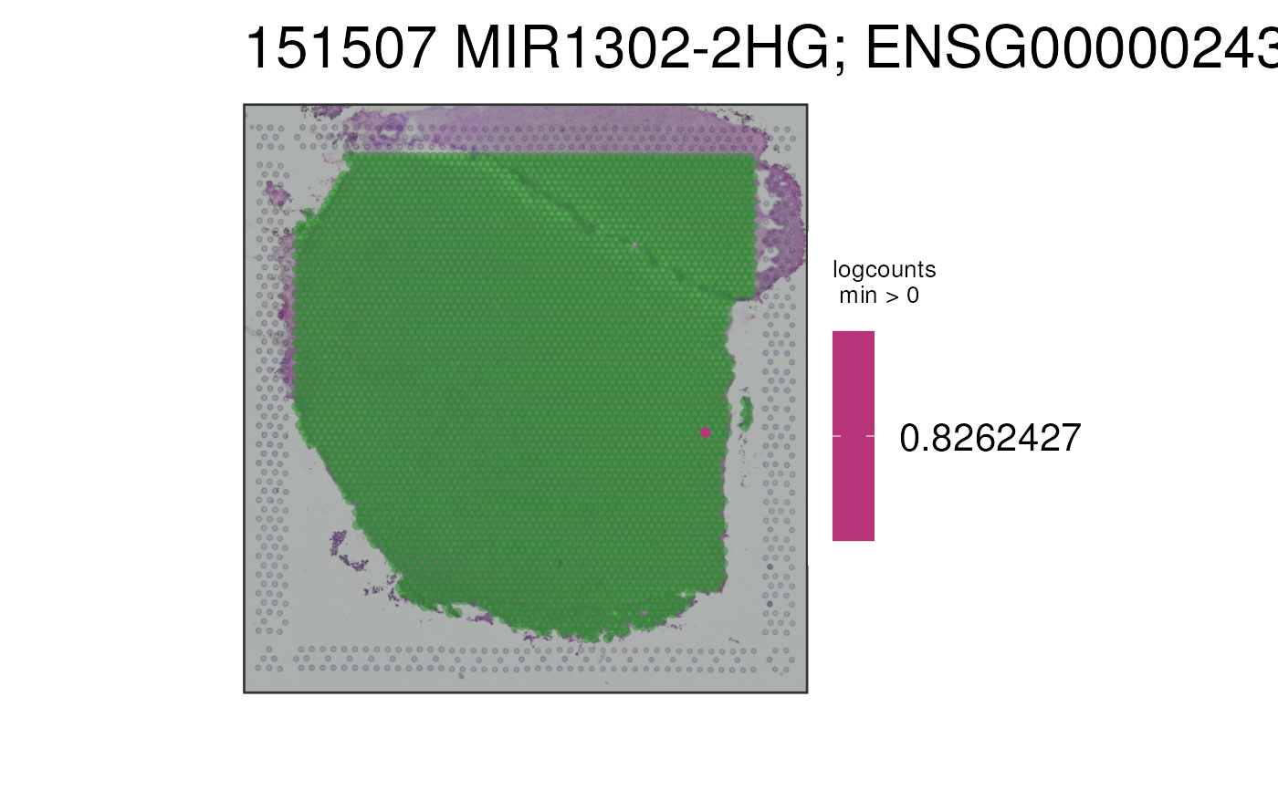
    ## Turn the alpha to NA, and use an alpha-blended "forestgreen" for
    ## the NA values
    # https://gist.githubusercontent.com/mages/5339689/raw/2aaa482dfbbecbfcb726525a3d81661f9d802a8e/add.alpha.R
    # add.alpha("forestgreen", 0.5)
    p2c <- vis_gene(
        spe = spe,
        sampleid = "151507",
        cont_colors = rev(viridisLite::viridis(21, option = "magma")),
        alpha = NA,
        na_color = "#228B2280"
    )
    print(p2c)

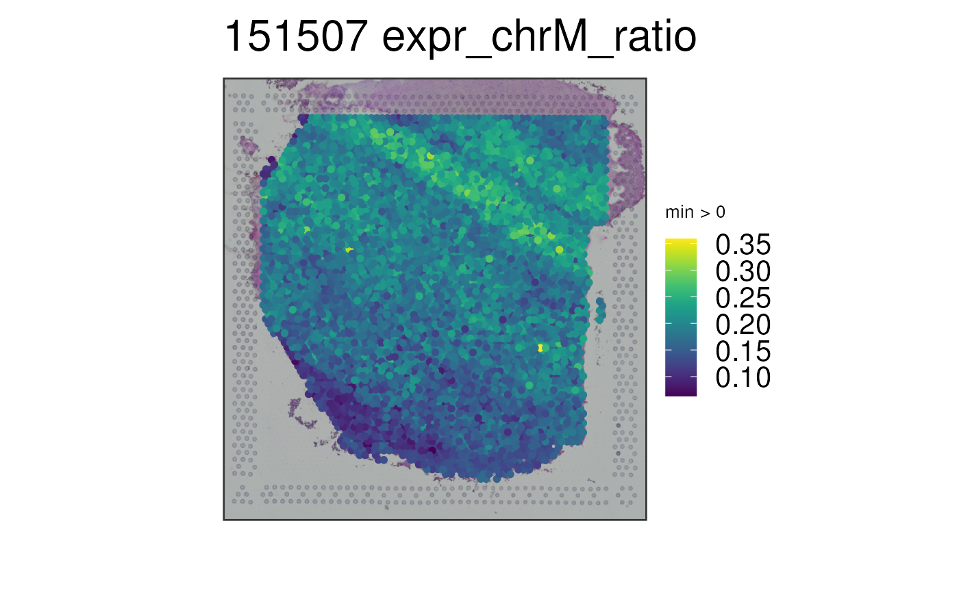
    ## Visualize a continuous variable, in this case, the ratio of chrM
    ## gene expression compared to the total expression at the spot-level
    p3 <- vis_gene(
        spe = spe,
        sampleid = "151507",
        geneid = "expr_chrM_ratio"
    )
    print(p3)

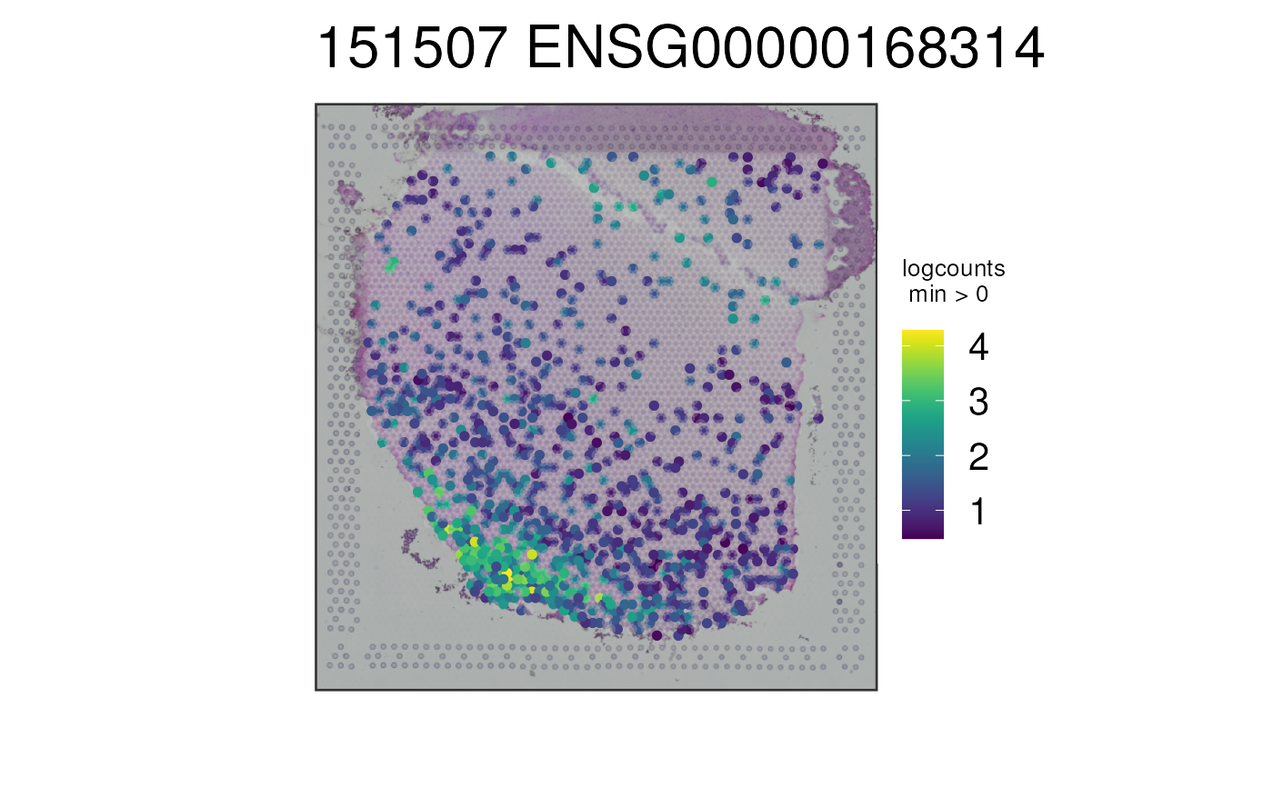
    ## Visualize a gene using the rownames(spe)
    p4 <- vis_gene(
        spe = spe,
        sampleid = "151507",
        geneid = rownames(spe)[which(rowData(spe)$gene_name == "MOBP")]
    )
    print(p4)

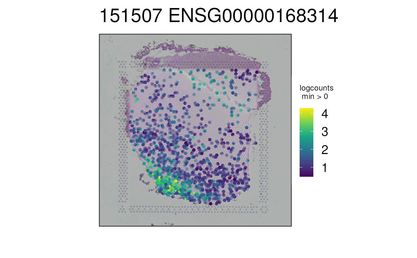
    ## Repeat without auto-cropping the image
    p5 <- vis_gene(
        spe = spe,
        sampleid = "151507",
        geneid = rownames(spe)[which(rowData(spe)$gene_name == "MOBP")],
        auto_crop = FALSE
    )
    print(p5)

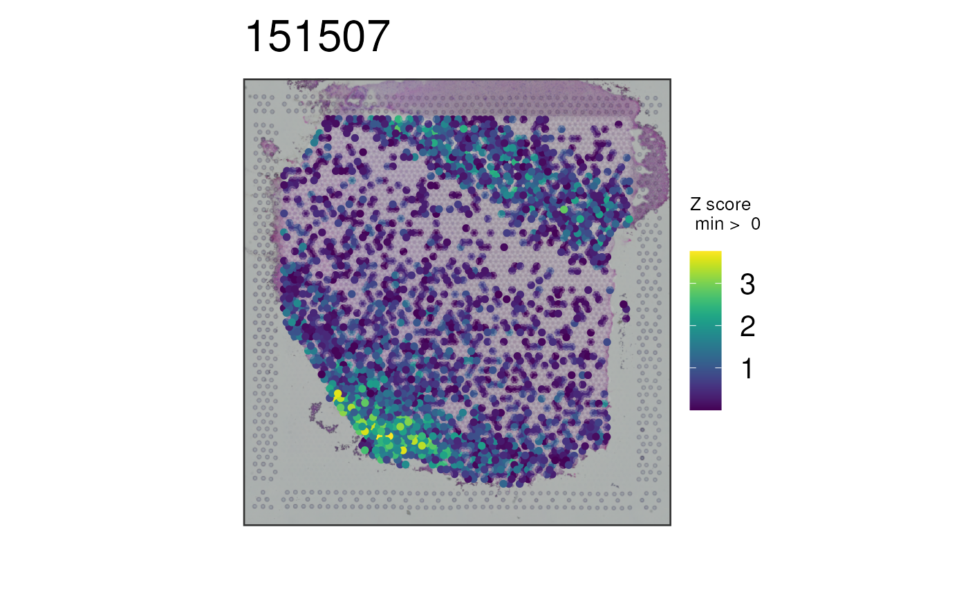
    #    Define several markers for white matter
    white_matter_genes <- c(
        "ENSG00000197971", "ENSG00000131095", "ENSG00000123560",
        "ENSG00000171885"
    )

    ## Plot all white matter markers at once using the Z-score combination
    ## method. Flatten this quantity at the top 5% of values for plotting
    p6 <- vis_gene(
        spe = spe,
        sampleid = "151507",
        geneid = white_matter_genes,
        multi_gene_method = "z_score",
        cap_percentile = 0.95
    )
    print(p6)

    ## Plot all white matter markers at once using the sparsity combination
    ## method
    p7 <- vis_gene(
        spe = spe,
        sampleid = "151507",
        geneid = white_matter_genes,
        multi_gene_method = "sparsity"
    )
    print(p7)

    ## Plot all white matter markers at once using the PCA combination
    ## method
    p8 <- vis_gene(
        spe = spe,
        sampleid = "151507",
        geneid = white_matter_genes,
        multi_gene_method = "pca"
    )
    print(p8)
}
#> 2025-05-09 16:32:02.404518 loading file /github/home/.cache/R/BiocFileCache/71157c99f803_Human_DLPFC_Visium_processedData_sce_scran_spatialLIBD.Rdata%3Fdl%3D1

Arguments

Value

Details

See also

Examples