Introduction to qsvaR
Joshua M. Stolz
Lieber Institute for Brain Developmentjstolz80@gmail.com
Hedia Tnani
Lieber Institute for Brain Developmenthediatnani0@gmail.com
Leonardo Collado-Torres
Lieber Institute for Brain Developmentlcolladotor@gmail.com
30 September 2025
Source:vignettes/Intro_qsvaR.Rmd
Intro_qsvaR.RmdBasics
Install qsvaR
R is an open-source statistical environment which can be
easily modified to enhance its functionality via packages. qsvaR is a
R package available via the Bioconductor repository for packages.
R can be installed on any operating system from CRAN after which you can install
qsvaR by
using the following commands in your R session:
## To install Bioconductor packages
if (!requireNamespace("BiocManager", quietly = TRUE)) {
    install.packages("BiocManager")
}

BiocManager::install("qsvaR")

## Check that you have a valid Bioconductor installation
BiocManager::valid()

## You can install the development version from GitHub with:
BiocManager::install("LieberInstitute/qsvaR")
Required knowledge
qsvaR is based on many other packages and in particular in those that have implemented the infrastructure needed for dealing with RNA-seq data. That is, packages like SummarizedExperiment. Here it might be useful for you to check the qSVA framework manuscript (Jaffe et al, PNAS, 2017).
If you are asking yourself the question “Where do I start using Bioconductor?” you might be interested in this blog post.
Asking for help
As package developers, we try to explain clearly how to use our
packages and in which order to use the functions. But R and
Bioconductor have a steep learning curve so it is critical
to learn where to ask for help. The blog post quoted above mentions some
but we would like to highlight the Bioconductor support site
as the main resource for getting help: remember to use the
qsvaR tag and check the older posts.
Other alternatives are available such as creating GitHub issues and
tweeting. However, please note that if you want to receive help you
should adhere to the posting
guidelines. It is particularly critical that you provide a small
reproducible example and your session information so package developers
can track down the source of the error.
Citing qsvaR
We hope that qsvaR will be useful for your research. Please use the following information to cite the package and the overall approach. Thank you!
## Citation info
citation("qsvaR")
#> To cite package 'qsvaR' in publications use:
#>
#>   Stolz JM, Tnani H, Collado-Torres L (2025). _qsvaR_.
#>   doi:10.18129/B9.bioc.qsvaR <https://doi.org/10.18129/B9.bioc.qsvaR>,
#>   https://github.com/LieberInstitute/qsvaR/qsvaR - R package version
#>   1.13.3, <http://www.bioconductor.org/packages/qsvaR>.
#>
#>   Stolz JM, Tnani H, Tao R, Jaffe AE, Collado-Torres L (2025). "qsvaR."
#>   _bioRxiv_. doi:10.1101/TODO <https://doi.org/10.1101/TODO>,
#>   <https://www.biorxiv.org/content/10.1101/TODO>.
#>
#> To see these entries in BibTeX format, use 'print(<citation>,
#> bibtex=TRUE)', 'toBibtex(.)', or set
#> 'options(citation.bibtex.max=999)'.
qsvaR Overview
Significant Transcripts
Differential expressions analysis requires the ability normalize complex datasets. In the case of postmortem brain tissue we are tasked with removing the effects of bench degradation. Our current work expands the scope of qSVA by generating degradation profiles (5 donors across 4 degradation time points: 0, 15, 30, and 60 minutes) from six human brain regions (n = 20 * 6 = 120): dorsolateral prefrontal cortex (DLPFC), hippocampus (HPC), medial prefrontal cortex (mPFC), subgenual anterior cingulate cortex (sACC), caudate, amygdala (AMY). We identified an average of 80,258 transcripts associated (FDR < 5%) with degradation time across the six brain regions. Testing for an interaction between brain region and degradation time identified 45,712 transcripts (FDR < 5%). A comparison of regions showed a unique pattern of expression changes associated with degradation time particularly in the DLPFC, implying that this region may not be representative of the effects of degradation on gene expression in other tissues. Furthermore previous work was done by analyzing expressed regions (Collado-Torres et al, NAR, 2017), and while this is an effective method of analysis, expressed regions are not a common output for many pipelines and are computationally expensive to identify, thus creating a barrier for the use of any qSVA software. In our most recent work expression quantification was performed at the transcript level using Salmon (Patro et al, Nat Methods, 2017). The changes from past work on qSVs to now is illustrated in the below cartoon.
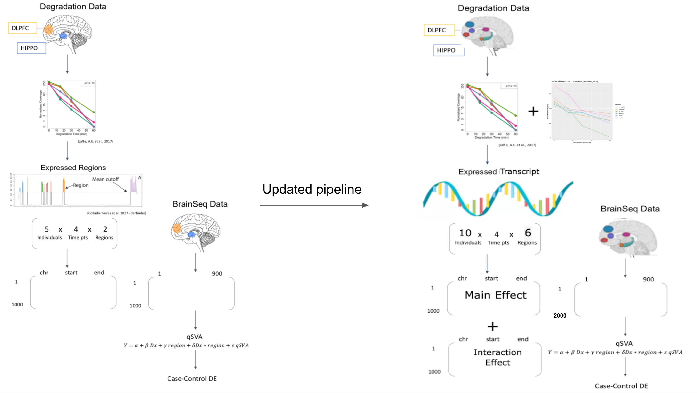
The diagram on the right shows the 2016 experimental design for qSVA.The diagram on the right shows the 2022 experimental design for qSVA.
The qsvaR
(Stolz, Tnani, and Collado-Torres, 2025) package combines an established
method for removing the effects of degradation from RNA-seq data with
easy to use functions. The first step in this workflow is to create an
RangedSummarizedExperiment
object with the transcripts identified in our qSVA experiment. If you
already have a RangedSummarizedExperiment
of transcripts we can do this with the getDegTx() function
as shown below.If not this can be generated with the
SPEAQeasy (a RNA-seq pipeline maintained by our lab)
pipeline usinge the --qsva flag. If you already have a RangedSummarizedExperiment
object with transcripts then you do not need to run
SPEAQeasy. This flag requires a full path to a text file,
containing one Ensembl transcript ID per line for each transcript
desired in the final transcripts R output object (called
rse_tx). The sig_transcripts argument in this
package should contain the same Ensembl transcript IDs as the text file
for the --qsva flag. The goal of qsvaR is to
provide software that can remove the effects of bench degradation from
RNA-seq data.
bfc <- BiocFileCache::BiocFileCache()

## Download brainseq phase 2 ##
rse_file <- BiocFileCache::bfcrpath(
    "https://s3.us-east-2.amazonaws.com/libd-brainseq2/rse_tx_unfiltered.Rdata",
    x = bfc
)
load(rse_file, verbose = TRUE)
#> Loading objects:
#>   rse_tx
## keep only adult samples and apply minimum expression cutoff
rse_tx <- rse_tx[, rse_tx$Age > 17]
rse_tx <- rse_tx[rowMeans(assays(rse_tx)$tpm) > 0.3, ]
Get Degradation Matrix
In this next step we subset for the transcripts associated with
degradation. These were determined by Joshua M. Stolz et al, 2022. We
have provided three models to choose from. Here the names
"cell_component", "top1500", and
"top1000" refer to models that were determined to be
effective in removing degradation effects. The "top1000"
model involves taking the union of the top 1000 transcripts associated
with degradation from the interaction model and the main effect model.
The "top1500" model is the same as the
"top1000" model except the union of the top 1500 genes
associated with degradation is selected. The most effective of our
models, "cell_component", involved deconvolution of the
degradation matrix to determine the proportion of cell types within our
studied tissue. These proportions were then added to our
model.matrix() and the union of the top 1000 transcripts in
the interaction model, the main effect model, and the cell proportions
model were used to generate this model of quality surrogate variables
(qSVs). In this example we will choose "cell_component"
when using the getDegTx() and
select_transcripts() functions.
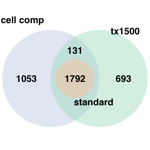
The above venn diagram shows the overlap between transcripts in each of the previously mentioned models.
# obtain transcripts with degradation signature
DegTx <- getDegTx(
  rse_tx, sig_transcripts = select_transcripts(cell_component = TRUE)
)
#> Using 2315 degradation-associated transcripts.
dim(DegTx)
#> [1] 2315  755
Generate principal components
The qSVs are derived from taking the principal components (PCs) of
the selected transcript expression data. This can be done with the
function getPCs. qSVs are essentially pricipal components
from an rna-seq experiment designed to model bench degradation. For more
on principal components you can read and introductory article here.
rse_tx specifies a RangedSummarizedExperiment
object that has the specified degraded transcripts. For us this is
DegTx. Here tpm is the name of the assay we
are using within the RangedSummarizedExperiment
object, where TPM stands for transcripts per million.
pcTx <- getPCs(rse_tx = DegTx, assayname = "tpm")Calculate Number of PCs Needed
Next we use the k_qsvs() function to calculate how many
PCs we will need to account for the variation. A model matrix accounting
for relevant variables should be used. Common variables such as Age,
Sex, Race and Religion are often included in the model. Again we are
using our RangedSummarizedExperiment DegTx as
the rse_tx option. Next we specify the mod
with our model.matrix(). model.matrix()
creates a design (or model) matrix, e.g., by expanding factors to a set
of dummy variables (depending on the contrasts) and expanding
interactions similarly. For more information on creating a design matrix
for your experiment see the documentation here.
Again we use the assayname option to specify that we are
using the tpm assay.
# design a basic model matrix to model the number of pcs needed
mod <- model.matrix(~ Dx + Age + Sex + Race + Region,
    data = colData(rse_tx)
)

## To ensure that the results are reproducible, you will need to set a
## random seed with the set.seed() function. Internally, we are using
## sva::num.sv() which needs a random seed to ensure reproducibility of the
## results.
set.seed(20230621)

# use k qsvs function to return a integer of pcs needed
k <- k_qsvs(rse_tx = DegTx, mod = mod, assayname = "tpm")
print(k)
#> [1] 19
Return qSV Matrix
Finally we subset our data to the calculated number of PCs. The
output of this function will be the qsvs for each sample. Here we use
the qsvPCs argument to enter the principal components
(pcTx). Here the argument k is the number of PCs we are
going to include as calculated in the previous step.
# get_qsvs use k to subset our pca analysis
qsvs <- get_qsvs(qsvPCs = pcTx, k = k)
dim(qsvs)
#> [1] 755  19
This can be done in one step with our wrapper function
qSVA which just combinds all the previous mentioned
functions.
## To ensure that the results are reproducible, you will need to set a
## random seed with the set.seed() function. Internally, we are using
## sva::num.sv() which needs a random seed to ensure reproducibility of the
## results.
set.seed(20230621)

## Example use of the wrapper function qSVA()
qsvs_wrapper <- qSVA(
    rse_tx = rse_tx,
    sig_transcripts = select_transcripts(cell_component = TRUE),
    mod = mod,
    assayname = "tpm"
)
#> Using 2315 degradation-associated transcripts.
dim(qsvs_wrapper)
#> [1] 755  19
Differential Expression
Next we can use a standard limma package approach to do differential
expression on the data. The key here is that we add our qsvs to the
model.matrix(). Here we input our
RangedSummarizedExperiment object and our
model.matrix() with qSVs. Note here that the
RangedSummarizedExperiment object is the original object
loaded with the full list of transcripts, not the the one we subsetted
for qSVs. This is because while PCs can be generated from a subset of
genes, differential expression is best done on the full dataset. The
expected output is a sigTx object that shows the results of
differential expression.
# create a model.matrix with demographic info and qsvs
mod_qSVA <- cbind(mod, qsvs)

# log tranform transcript expression
txExprs <- log2(assays(rse_tx)$tpm + 1)

# linear model differential expression
fitTx <- lmFit(txExprs, mod_qSVA)

# generate empirical bayes for DE
eBTx <- eBayes(fitTx)

# get DE results table
sigTx <- topTable(eBTx,
    coef = 2,
    p.value = 1, number = nrow(rse_tx)
)
head(sigTx)
#>                         logFC  AveExpr         t      P.Value    adj.P.Val
#> ENST00000484223.1 -0.16801225 1.155197 -6.434391 2.241717e-10 2.253733e-05
#> ENST00000344423.9  0.08388265 1.823057  6.023398 2.705136e-09 1.359818e-04
#> ENST00000453370.1 -0.14813207 1.405052 -5.578121 3.424946e-08 1.060144e-03
#> ENST00000399808.4  0.24131361 4.393914  5.540228 4.217967e-08 1.060144e-03
#> ENST00000373510.8  0.03789957 1.274950  5.486733 5.647882e-08 1.135631e-03
#> ENST00000446193.1 -0.12094546 2.303149 -5.277337 1.729461e-07 2.663972e-03
#>                           B
#> ENST00000484223.1 13.199862
#> ENST00000344423.9 10.837738
#> ENST00000453370.1  8.437965
#> ENST00000399808.4  8.241509
#> ENST00000373510.8  7.966261
#> ENST00000446193.1  6.912510
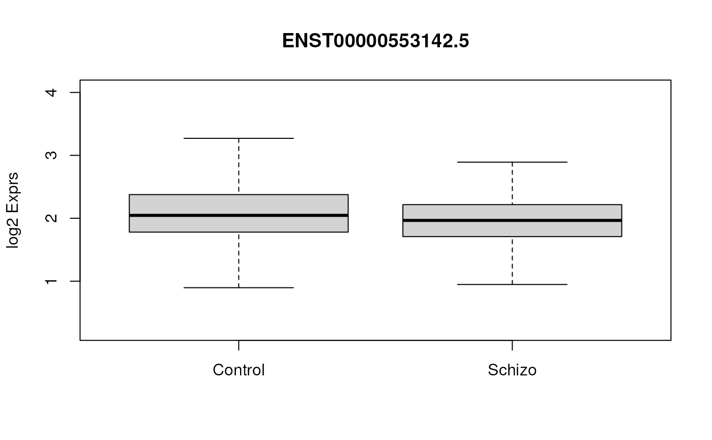
If we look at a plot of our most significant transcript we can see that at this level we don’t have that much fold change in our data at any individual transcript. These transcripts are however significant and it might be valuable to repeat the analysis at gene level. At gene level the results can be used to do gene ontology enrichment with packages such as clusterProfiler.
# get expression for most significant gene
yy <- txExprs[rownames(txExprs) == rownames(sigTx)[1], ]

## Visualize the expression of this gene using boxplots
p <- boxplot(yy ~ rse_tx$Dx,
    outline = FALSE,
    ylim = range(yy), ylab = "log2 Exprs", xlab = "",
    main = paste(rownames(sigTx)[1])
)
We can assess the effectiveness of our analysis by first performing DE without qSVs
# log tranform transcript expression
txExprs_noqsv <- log2(assays(rse_tx)$tpm + 1)

# linear model differential expression with generic model
fitTx_noqsv <- lmFit(txExprs_noqsv, mod)

# generate empirical bayes for DE
eBTx_noqsv <- eBayes(fitTx_noqsv)

# get DE results table
sigTx_noqsv <- topTable(eBTx_noqsv,
    coef = 2,
    p.value = 1, number = nrow(rse_tx)
)

## Explore the top results
head(sigTx_noqsv)
#>                        logFC   AveExpr         t      P.Value    adj.P.Val
#> ENST00000550948.1 -0.3354760 1.4286901 -8.476210 1.225373e-16 6.726210e-12
#> ENST00000399220.2 -0.4971139 1.8855923 -8.456466 1.430341e-16 6.726210e-12
#> ENST00000302632.3 -0.5085661 2.7498973 -8.413088 2.007105e-16 6.726210e-12
#> ENST00000540372.5 -0.1841983 0.5557803 -8.048071 3.284430e-15 8.255086e-11
#> ENST00000412814.1 -0.2602673 0.6388824 -7.785603 2.302633e-14 4.629950e-10
#> ENST00000237612.7 -0.2891861 2.3009743 -7.558877 1.186468e-13 1.988046e-09
#>                          B
#> ENST00000550948.1 26.83858
#> ENST00000399220.2 26.69150
#> ENST00000302632.3 26.36938
#> ENST00000540372.5 23.71308
#> ENST00000412814.1 21.86396
#> ENST00000237612.7 20.30843
Next we should subset our differential expression output to just the t-statistic
## Subset the topTable() results to keep just the t-statistic
DE_noqsv <- data.frame(t = sigTx_noqsv$t, row.names = rownames(sigTx_noqsv))
DE <- data.frame(t = sigTx$t, row.names = rownames(sigTx))

## Explore this data.frame()
head(DE)
#>                           t
#> ENST00000484223.1 -6.434391
#> ENST00000344423.9  6.023398
#> ENST00000453370.1 -5.578121
#> ENST00000399808.4  5.540228
#> ENST00000373510.8  5.486733
#> ENST00000446193.1 -5.277337
Using our DEqual function we can make a plot comparing
the t-statistics from degradation and our differential expression
output. In the first model below there is a 0.5 correlation between
degradation t-statistics and our differential expression. This means the
data is likely confounded for degradation and will lead to many false
positives.
## Generate a DEqual() plot using the model results without qSVs
DEqual(DE_noqsv)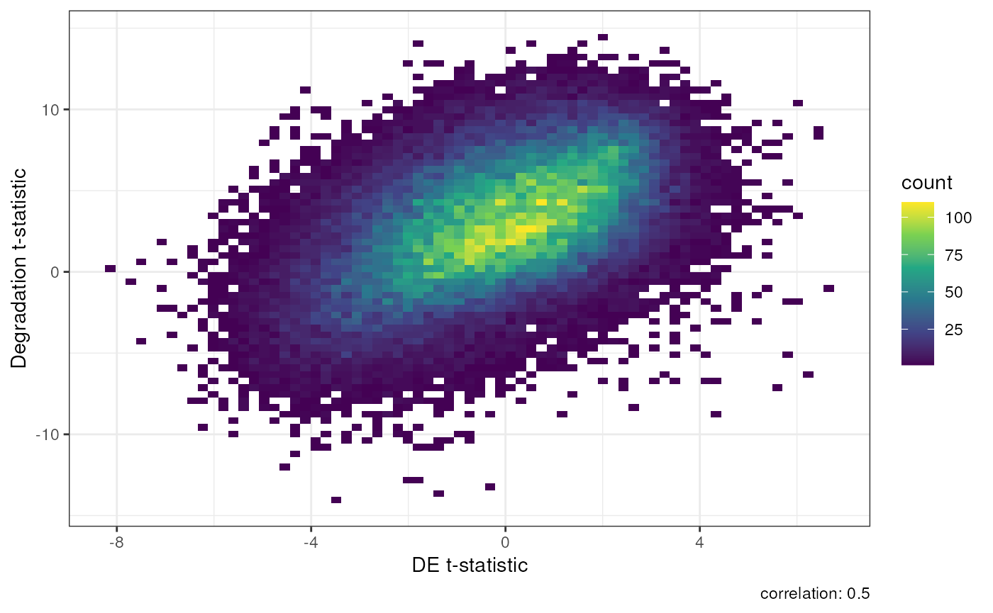
Result of Differential Expression without qSVA normalization.
In the plot below when we add qSVs to our model we reduce the association with degradation to -0.014, which is very close to 0.
## Generate a DEqual() plot using the model results with qSVs
DEqual(DE)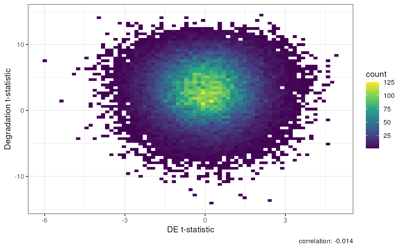
Result of Differential Expression with qSVA normalization.
Conclusion
We have shown that this method is effective for removing the effects of degradation from RNA-seq data. We found that the qsvaR is simpler to use than the previous version from 2016 that used expressed regions instead of transcripts making this software package preferable for users. I would encourage users to read how each set of degradation transcripts was selected as not all models may be appropriate for every experiment. Thank you for your interest and for using qsvaR (Stolz, Tnani, and Collado-Torres, 2025)!
Acknowledgements
We would like to thank:
- Heena Divecha for proofreading the documentation of qsvaR
- Louise A. Huuki-Myers for guidance with understanding R code and editing qsvaR
-
Nicholas J. Eagles for
help processing RNA-seq data with
SPEAQeasy - Aja Hope for proofreading the documentation of qsvaR
Reproducibility
The qsvaR package (Stolz, Tnani, and Collado-Torres, 2025) was made possible thanks to:
- R (R Core Team, 2024)
- BiocFileCache (Shepherd and Morgan, 2024)
- BiocStyle (Oleś, 2024)
- covr (Hester, 2023)
- ggplot2 (Wickham, 2016)
- knitr (Xie, 2025)
- limma (Ritchie, Phipson, Wu, Hu, Law, Shi, and Smyth, 2015)
- RefManageR (McLean, 2017)
- rmarkdown (Allaire, Xie, Dervieux, McPherson, Luraschi, Ushey, Atkins, Wickham, Cheng, Chang, and Iannone, 2025)
- sessioninfo (Wickham, Chang, Flight, Müller, and Hester, 2025)
- testthat (Wickham, 2011)
- SummarizedExperiment (Morgan, Obenchain, Hester, and Pagès, 2024)
- sva (Leek, Johnson, Parker, Fertig, Jaffe, Zhang, Storey, and Torres, 2024)
This package was developed using biocthis.
Code for creating the vignette
## Create the vignette
library("rmarkdown")
system.time(render("Intro_qsvaR.Rmd", "BiocStyle::html_document"))

## Extract the R code
library("knitr")
knit("Intro_qsvaR.Rmd", tangle = TRUE)
Date the vignette was generated.
#> [1] "2025-09-30 02:09:50 UTC"Wallclock time spent generating the vignette.
#> Time difference of 56.551 secsR session information.
#> ─ Session info ───────────────────────────────────────────────────────────────────────────────────────────────────────
#>  setting  value
#>  version  R version 4.4.2 (2024-10-31)
#>  os       Ubuntu 24.04.1 LTS
#>  system   x86_64, linux-gnu
#>  ui       X11
#>  language en
#>  collate  en_US.UTF-8
#>  ctype    en_US.UTF-8
#>  tz       UTC
#>  date     2025-09-30
#>  pandoc   3.6 @ /usr/bin/ (via rmarkdown)
#>  quarto   1.5.57 @ /usr/local/bin/quarto
#>
#> ─ Packages ───────────────────────────────────────────────────────────────────────────────────────────────────────────
#>  package              * version   date (UTC) lib source
#>  abind                  1.4-8     2024-09-12 [1] RSPM (R 4.4.0)
#>  annotate               1.84.0    2024-10-29 [1] Bioconductor 3.20 (R 4.4.2)
#>  AnnotationDbi          1.68.0    2024-10-29 [1] Bioconductor 3.20 (R 4.4.2)
#>  backports              1.5.0     2024-05-23 [1] RSPM (R 4.4.0)
#>  bibtex                 0.5.1     2023-01-26 [1] RSPM (R 4.4.0)
#>  Biobase              * 2.66.0    2024-10-29 [1] Bioconductor 3.20 (R 4.4.2)
#>  BiocFileCache        * 2.14.0    2024-10-29 [1] Bioconductor 3.20 (R 4.4.2)
#>  BiocGenerics         * 0.52.0    2024-10-29 [1] Bioconductor 3.20 (R 4.4.2)
#>  BiocManager            1.30.26   2025-06-05 [1] RSPM (R 4.4.0)
#>  BiocParallel           1.40.2    2025-09-26 [1] Bioconductor
#>  BiocStyle            * 2.34.0    2024-10-29 [1] Bioconductor 3.20 (R 4.4.2)
#>  Biostrings             2.74.1    2024-12-16 [1] Bioconductor 3.20 (R 4.4.2)
#>  bit                    4.6.0     2025-03-06 [1] RSPM (R 4.4.0)
#>  bit64                  4.6.0-1   2025-01-16 [1] RSPM (R 4.4.0)
#>  blob                   1.2.4     2023-03-17 [1] RSPM (R 4.4.0)
#>  bookdown               0.44      2025-08-21 [1] RSPM (R 4.4.0)
#>  bslib                  0.9.0     2025-01-30 [2] RSPM (R 4.4.0)
#>  cachem                 1.1.0     2024-05-16 [2] RSPM (R 4.4.0)
#>  cli                    3.6.5     2025-04-23 [2] RSPM (R 4.4.0)
#>  codetools              0.2-20    2024-03-31 [3] CRAN (R 4.4.2)
#>  crayon                 1.5.3     2024-06-20 [2] RSPM (R 4.4.0)
#>  curl                   7.0.0     2025-08-19 [2] RSPM (R 4.4.0)
#>  DBI                    1.2.3     2024-06-02 [1] RSPM (R 4.4.0)
#>  dbplyr               * 2.5.1     2025-09-10 [1] RSPM (R 4.4.0)
#>  DelayedArray           0.32.0    2024-10-29 [1] Bioconductor 3.20 (R 4.4.2)
#>  desc                   1.4.3     2023-12-10 [2] RSPM (R 4.4.0)
#>  digest                 0.6.37    2024-08-19 [2] RSPM (R 4.4.0)
#>  dplyr                  1.1.4     2023-11-17 [1] RSPM (R 4.4.0)
#>  edgeR                  4.4.2     2025-01-27 [1] Bioconductor 3.20 (R 4.4.2)
#>  evaluate               1.0.5     2025-08-27 [2] RSPM (R 4.4.0)
#>  farver                 2.1.2     2024-05-13 [1] RSPM (R 4.4.0)
#>  fastmap                1.2.0     2024-05-15 [2] RSPM (R 4.4.0)
#>  filelock               1.0.3     2023-12-11 [1] RSPM (R 4.4.0)
#>  fs                     1.6.6     2025-04-12 [2] RSPM (R 4.4.0)
#>  genefilter             1.88.0    2024-10-29 [1] Bioconductor 3.20 (R 4.4.2)
#>  generics               0.1.4     2025-05-09 [1] RSPM (R 4.4.0)
#>  GenomeInfoDb         * 1.42.3    2025-01-27 [1] Bioconductor 3.20 (R 4.4.2)
#>  GenomeInfoDbData       1.2.13    2025-03-08 [1] Bioconductor
#>  GenomicRanges        * 1.58.0    2024-10-29 [1] Bioconductor 3.20 (R 4.4.2)
#>  ggplot2                4.0.0     2025-09-11 [1] RSPM (R 4.4.0)
#>  glue                   1.8.0     2024-09-30 [2] RSPM (R 4.4.0)
#>  gtable                 0.3.6     2024-10-25 [1] RSPM (R 4.4.0)
#>  htmltools              0.5.8.1   2024-04-04 [2] RSPM (R 4.4.0)
#>  htmlwidgets            1.6.4     2023-12-06 [2] RSPM (R 4.4.0)
#>  httr                   1.4.7     2023-08-15 [1] RSPM (R 4.4.0)
#>  IRanges              * 2.40.1    2024-12-05 [1] Bioconductor 3.20 (R 4.4.2)
#>  jquerylib              0.1.4     2021-04-26 [2] RSPM (R 4.4.0)
#>  jsonlite               2.0.0     2025-03-27 [2] RSPM (R 4.4.0)
#>  KEGGREST               1.46.0    2024-10-29 [1] Bioconductor 3.20 (R 4.4.2)
#>  knitr                  1.50      2025-03-16 [2] RSPM (R 4.4.0)
#>  labeling               0.4.3     2023-08-29 [1] RSPM (R 4.4.0)
#>  lattice                0.22-7    2025-04-02 [3] RSPM (R 4.4.0)
#>  lifecycle              1.0.4     2023-11-07 [2] RSPM (R 4.4.0)
#>  limma                * 3.62.2    2025-01-09 [1] Bioconductor 3.20 (R 4.4.2)
#>  locfit                 1.5-9.12  2025-03-05 [1] RSPM (R 4.4.0)
#>  lubridate              1.9.4     2024-12-08 [1] RSPM (R 4.4.0)
#>  magrittr               2.0.4     2025-09-12 [2] RSPM (R 4.4.0)
#>  Matrix                 1.7-4     2025-08-28 [3] RSPM (R 4.4.0)
#>  MatrixGenerics       * 1.18.1    2025-01-09 [1] Bioconductor 3.20 (R 4.4.2)
#>  matrixStats          * 1.5.0     2025-01-07 [1] RSPM (R 4.4.0)
#>  memoise                2.0.1     2021-11-26 [2] RSPM (R 4.4.0)
#>  mgcv                   1.9-3     2025-04-04 [3] RSPM (R 4.4.0)
#>  nlme                   3.1-168   2025-03-31 [3] RSPM (R 4.4.0)
#>  pillar                 1.11.1    2025-09-17 [2] RSPM (R 4.4.0)
#>  pkgconfig              2.0.3     2019-09-22 [2] RSPM (R 4.4.0)
#>  pkgdown                2.1.3     2025-05-25 [2] RSPM (R 4.4.0)
#>  plyr                   1.8.9     2023-10-02 [1] RSPM (R 4.4.0)
#>  png                    0.1-8     2022-11-29 [1] RSPM (R 4.4.0)
#>  purrr                  1.1.0     2025-07-10 [2] RSPM (R 4.4.0)
#>  qsvaR                * 1.13.3    2025-09-30 [1] Bioconductor
#>  R6                     2.6.1     2025-02-15 [2] RSPM (R 4.4.0)
#>  ragg                   1.5.0     2025-09-02 [2] RSPM (R 4.4.0)
#>  RColorBrewer           1.1-3     2022-04-03 [1] RSPM (R 4.4.0)
#>  Rcpp                   1.1.0     2025-07-02 [2] RSPM (R 4.4.0)
#>  RefManageR           * 1.4.0     2022-09-30 [1] RSPM (R 4.4.0)
#>  rlang                  1.1.6     2025-04-11 [2] RSPM (R 4.4.0)
#>  rmarkdown              2.30      2025-09-28 [2] RSPM (R 4.4.0)
#>  RSQLite                2.4.3     2025-08-20 [1] RSPM (R 4.4.0)
#>  S4Arrays               1.6.0     2024-10-29 [1] Bioconductor 3.20 (R 4.4.2)
#>  S4Vectors            * 0.44.0    2024-10-29 [1] Bioconductor 3.20 (R 4.4.2)
#>  S7                     0.2.0     2024-11-07 [1] RSPM (R 4.4.0)
#>  sass                   0.4.10    2025-04-11 [2] RSPM (R 4.4.0)
#>  scales                 1.4.0     2025-04-24 [1] RSPM (R 4.4.0)
#>  sessioninfo          * 1.2.3     2025-02-05 [2] RSPM (R 4.4.0)
#>  SparseArray            1.6.2     2025-02-20 [1] Bioconductor 3.20 (R 4.4.2)
#>  statmod                1.5.0     2023-01-06 [1] RSPM (R 4.4.0)
#>  stringi                1.8.7     2025-03-27 [2] RSPM (R 4.4.0)
#>  stringr                1.5.2     2025-09-08 [2] RSPM (R 4.4.0)
#>  SummarizedExperiment * 1.36.0    2024-10-29 [1] Bioconductor 3.20 (R 4.4.2)
#>  survival               3.8-3     2024-12-17 [3] RSPM (R 4.4.0)
#>  sva                    3.54.0    2024-10-29 [1] Bioconductor 3.20 (R 4.4.2)
#>  systemfonts            1.2.3     2025-04-30 [2] RSPM (R 4.4.0)
#>  textshaping            1.0.3     2025-09-02 [2] RSPM (R 4.4.0)
#>  tibble                 3.3.0     2025-06-08 [2] RSPM (R 4.4.0)
#>  tidyselect             1.2.1     2024-03-11 [1] RSPM (R 4.4.0)
#>  timechange             0.3.0     2024-01-18 [1] RSPM (R 4.4.0)
#>  UCSC.utils             1.2.0     2024-10-29 [1] Bioconductor 3.20 (R 4.4.2)
#>  vctrs                  0.6.5     2023-12-01 [2] RSPM (R 4.4.0)
#>  viridisLite            0.4.2     2023-05-02 [1] RSPM (R 4.4.0)
#>  withr                  3.0.2     2024-10-28 [2] RSPM (R 4.4.0)
#>  xfun                   0.53      2025-08-19 [2] RSPM (R 4.4.0)
#>  XML                    3.99-0.19 2025-08-22 [1] RSPM (R 4.4.0)
#>  xml2                   1.4.0     2025-08-20 [2] RSPM (R 4.4.0)
#>  xtable                 1.8-4     2019-04-21 [2] RSPM (R 4.4.0)
#>  XVector                0.46.0    2024-10-29 [1] Bioconductor 3.20 (R 4.4.2)
#>  yaml                   2.3.10    2024-07-26 [2] RSPM (R 4.4.0)
#>  zlibbioc               1.52.0    2024-10-29 [1] Bioconductor 3.20 (R 4.4.2)
#>
#>  [1] /__w/_temp/Library
#>  [2] /usr/local/lib/R/site-library
#>  [3] /usr/local/lib/R/library
#>  * ── Packages attached to the search path.
#>
#> ──────────────────────────────────────────────────────────────────────────────────────────────────────────────────────
Bibliography
This vignette was generated using BiocStyle (Oleś, 2024) with knitr (Xie, 2025) and rmarkdown (Allaire, Xie, Dervieux et al., 2025) running behind the scenes.
Citations made with RefManageR (McLean, 2017).
[1] J. Allaire, Y. Xie, C. Dervieux, et al. rmarkdown: Dynamic Documents for R. R package version 2.30. 2025. URL: https://github.com/rstudio/rmarkdown.
[2] J. Hester. covr: Test Coverage for Packages. R package version 3.6.4, https://github.com/r-lib/covr. 2023. URL: https://covr.r-lib.org.
[3] J. T. Leek, W. E. Johnson, H. S. Parker, et al. sva: Surrogate Variable Analysis. R package version 3.54.0. 2024. DOI: 10.18129/B9.bioc.sva. URL: https://bioconductor.org/packages/sva.
[4] M. W. McLean. “RefManageR: Import and Manage BibTeX and BibLaTeX References in R”. In: The Journal of Open Source Software (2017). DOI: 10.21105/joss.00338.
[5] M. Morgan, V. Obenchain, J. Hester, et al. SummarizedExperiment: A container (S4 class) for matrix-like assays. R package version 1.36.0. 2024. DOI: 10.18129/B9.bioc.SummarizedExperiment. URL: https://bioconductor.org/packages/SummarizedExperiment.
[6] A. Oleś. BiocStyle: Standard styles for vignettes and other Bioconductor documents. R package version 2.34.0. 2024. DOI: 10.18129/B9.bioc.BiocStyle. URL: https://bioconductor.org/packages/BiocStyle.
[7] R Core Team. R: A Language and Environment for Statistical Computing. R Foundation for Statistical Computing. Vienna, Austria, 2024. URL: https://www.R-project.org/.
[8] M. E. Ritchie, B. Phipson, D. Wu, et al. “limma powers differential expression analyses for RNA-sequencing and microarray studies”. In: Nucleic Acids Research 43.7 (2015), p. e47. DOI: 10.1093/nar/gkv007.
[9] L. Shepherd and M. Morgan. BiocFileCache: Manage Files Across Sessions. R package version 2.14.0. 2024. DOI: 10.18129/B9.bioc.BiocFileCache. URL: https://bioconductor.org/packages/BiocFileCache.
[10] J. M. Stolz, H. Tnani, and L. Collado-Torres. qsvaR. https://github.com/LieberInstitute/qsvaR/qsvaR - R package version 1.13.3. 2025. DOI: 10.18129/B9.bioc.qsvaR. URL: http://www.bioconductor.org/packages/qsvaR.
[11] H. Wickham. ggplot2: Elegant Graphics for Data Analysis. Springer-Verlag New York, 2016. ISBN: 978-3-319-24277-4. URL: https://ggplot2.tidyverse.org.
[12] H. Wickham. “testthat: Get Started with Testing”. In: The R Journal 3 (2011), pp. 5–10. URL: https://journal.r-project.org/archive/2011-1/RJournal_2011-1_Wickham.pdf.
[13] H. Wickham, W. Chang, R. Flight, et al. sessioninfo: R Session Information. R package version 1.2.3, https://sessioninfo.r-lib.org. 2025. URL: https://github.com/r-lib/sessioninfo#readme.
[14] Y. Xie. knitr: A General-Purpose Package for Dynamic Report Generation in R. R package version 1.50. 2025. URL: https://yihui.org/knitr/.