Differential expressions analysis requires the ability to normalize complex datasets. In the case of postmortem brain tissue we are tasked with removing the effects of bench degradation. The qsvaR package combines an established method for removing the effects of degradation from RNA-seq data with easy to use functions. It is the second iteration of the qSVA framework (Jaffe et al, PNAS, 2017).
The first step in the qsvaR workflow is to create an RangedSummarizedExperiment object with the transcripts identified in our qSVA experiment. If you already have a RangedSummarizedExperiment of transcripts we can do this with the getDegTx() function as shown below.If not this can be generated with the SPEAQeasy (a RNA-seq pipeline maintained by our lab) pipeline using the --qsva flag. If you already have a RangedSummarizedExperiment object with transcripts then you do not need to run SPEAQeasy. This flag requires a full path to a text file, containing one Ensembl transcript ID per line for each transcript desired in the final transcripts R output object (called rse_tx). The sig_transcripts argument in this package should contain the same Ensembl transcript IDs as the text file for the --qsva flag.The goal of qsvaR is to provide software that can remove the effects of bench degradation from RNA-seq data.
Installation Instructions
Get the latest stable R release from CRAN. Then install qsvaR using from Bioconductor the following code:
if (!requireNamespace("BiocManager", quietly = TRUE)) {
    install.packages("BiocManager")
}

BiocManager::install("qsvaR")
And the development version from GitHub with:
BiocManager::install("LieberInstitute/qsvaR")Example
This is a basic example which shows how to obtain the quality surrogate variables (qSVs) for the brainseq phase II dataset. qSVs are essentially principal components from an rna-seq experiment designed to model bench degradation. For more on principal components you can read and introductory article here. At the start of this script we will have an RangedSummarizedExperiment and a list of all the transcripts found in our degradation study. At the end we will have a table with differential expression results that is adjusted for qSVs.
library("qsvaR")

## We'll download example data from the BrainSeq Phase II project
## described at http://eqtl.brainseq.org/phase2/.
##
## We'll use BiocFileCache to cache these files so you don't have to download
## them again for other examples.
bfc <- BiocFileCache::BiocFileCache()
rse_file <- BiocFileCache::bfcrpath(
    "https://s3.us-east-2.amazonaws.com/libd-brainseq2/rse_tx_unfiltered.Rdata",
    x = bfc
)
#> adding rname 'https://s3.us-east-2.amazonaws.com/libd-brainseq2/rse_tx_unfiltered.Rdata'

## Now that we have the data in our computer, we can load it.
load(rse_file, verbose = TRUE)
#> Loading objects:
#>   rse_tx
In this next step, we subset to the transcripts associated with degradation. qsvaR provides significant transcripts determined in four different linear models of transcript expression against degradation time, brain region, and potentially cell-type proportions:
exp ~ DegradationTime + Regionexp ~ DegradationTime * Regionexp ~ DegradationTime + Region + CellTypePropexp ~ DegradationTime * Region + CellTypeProp
select_transcripts() returns degradation-associated transcripts and supports two parameters. First, top_n controls how many significant transcripts to extract from each model. When cell_component = TRUE, all four models are used; otherwise, just the first two are used. The union of significant transcripts from all used models is returned.
As an example, we’ll subset our RangedSummarizedExperiment to the union of the top 1000 significant transcripts derived from each of the four models.
#   Subset 'rse_tx' to the top 1000 significant transcripts from the four
#   degradation models
DegTx <- getDegTx(
    rse_tx,
    sig_transcripts = select_transcripts(top_n = 1000, cell_component = TRUE)
)
#> Using 2496 degradation-associated transcripts.

## Now we can compute the Principal Components (PCs) of the degraded
## transcripts
pcTx <- getPCs(DegTx, "tpm")
Next we use the k_qsvs() function to calculate how many PCs we will need to account for the variation. A model matrix accounting for relevant variables should be used. Common variables such as Age, Sex, Race and Region are often included in the model. Again we are using our RangedSummarizedExperiment DegTx as the rse_tx option. Next we specify the mod with our model.matrix(). model.matrix() creates a design (or model) matrix, e.g., by expanding factors to a set of dummy variables (depending on the contrasts) and expanding interactions similarly. For more information on creating a design matrix for your experiment see the documentation here. Again we use the assayname option to specify the we are using the tpm assay, where TPM stands for transcripts per million.
## Using a simple statistical model we determine the number of PCs needed (k)
mod <- model.matrix(~ Dx + Age + Sex + Race + Region,
    data = colData(rse_tx)
)
k <- k_qsvs(DegTx, mod, "tpm")
print(k)
#> [1] 20
Now that we have our PCs and the number we need we can generate our qSVs.
This can be done in one step with our wrapper function qSVA which just combinds all the previous mentioned functions.
## Example use of the wrapper function qSVA()
qsvs_wrapper <- qSVA(
    rse_tx = rse_tx,
    sig_transcripts = select_transcripts(top_n = 1000, cell_component = TRUE),
    mod = mod,
    assayname = "tpm"
)
#> Using 2496 degradation-associated transcripts.
dim(qsvs_wrapper)
#> [1] 900  20
Differential Expression
Next we can use a standard limma package approach to do differential expression on the data. The key here is that we add our qSVs to the statistical model we use through model.matrix(). Here we input our Ranged SummarizedExperiment object and our model.matrix with qSVs. Note here that the Ranged SummarizedExperiment object is the original object loaded with the full list of transcripts, not the the one we subsetted for qSVs. This is because while PCs can be generated from a subset of genes, differential expression is best done on the full dataset. The expected output is a sigTx object that shows the results of differential expression.
library("limma")

## Add the qSVs to our statistical model
mod_qSVA <- cbind(
    mod,
    qsvs
)

## Extract the transcript expression values and put them in the
## log2(TPM + 1) scale
txExprs <- log2(assays(rse_tx)$tpm + 1)

## Run the standard linear model for differential expression
fitTx <- lmFit(txExprs, mod_qSVA)
eBTx <- eBayes(fitTx)

## Extract the differential expression results
sigTx <- topTable(eBTx,
    coef = 2,
    p.value = 1, number = nrow(rse_tx)
)

## Explore the top results
head(sigTx)
#>                         logFC  AveExpr         t      P.Value    adj.P.Val
#> ENST00000484223.1 -0.17439018 1.144051 -6.685583 4.099898e-11 8.121610e-06
#> ENST00000344423.9  0.09212678 1.837102  6.449533 1.855943e-10 1.838246e-05
#> ENST00000399808.4  0.28974369 4.246788  6.320041 4.165237e-10 2.233477e-05
#> ENST00000467370.5  0.06313938 0.301711  6.307179 4.509956e-10 2.233477e-05
#> ENST00000264657.9  0.09913353 2.450684  5.933186 4.280565e-09 1.375288e-04
#> ENST00000415912.6  0.09028757 1.736581  5.918230 4.671963e-09 1.375288e-04
#>                           B
#> ENST00000484223.1 14.338379
#> ENST00000344423.9 12.865110
#> ENST00000399808.4 12.077344
#> ENST00000467370.5 11.999896
#> ENST00000264657.9  9.811110
#> ENST00000415912.6  9.726142
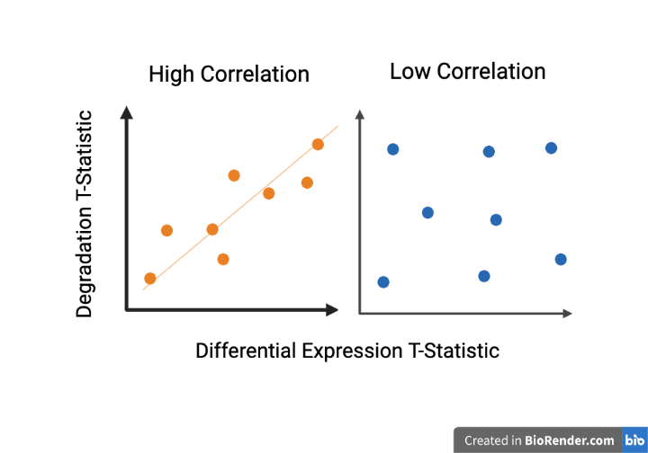
Finally, you can compare the resulting t-statistics from your differential expression model against the degradation time t-statistics adjusting for the six different brain regions. This type of plot is called DEqual plot and was shown in the initial qSVA framework paper (Jaffe et al, PNAS, 2017). We are really looking for two patterns exemplified here in Figure 1 (cartoon shown earlier). A direct positive correlation with degradation shown in Figure 1 on the right tells us that there is signal in the data associated with qSVs. An example of nonconfounded data or data that has been modeled can be seen in Figure 1 on the right with its lack of relationship between the x and y variables.

Cartoon showing patterns in DEqual plots
## Generate a DEqual() plot using the model results with qSVs
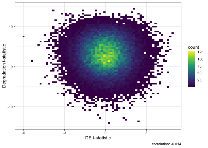
DEqual(sigTx)
Result of Differential Expression with qSVA normalization.
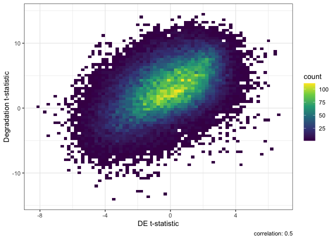
For comparison, here is the DEqual() plot for the model without qSVs.
## Generate a DEqual() plot using the model results without qSVs
DEqual(topTable(eBayes(lmFit(txExprs, mod)), coef = 2, p.value = 1, number = nrow(rse_tx)))
Result of Differential Expression without qSVA normalization.
In these two DEqual plots we can see that the first is much better. With a correlation of -0.014 we can effectively conclude that we have removed the effects of degradation from the data. In the second plot after modeling for several common variables we still have a correlation of 0.5 with the degradation experiment. This high correlation shows we still have a large amount of signal from degradation in our data potentially confounding our case-control (SCZD vs neurotypical controls) differential expression results.


