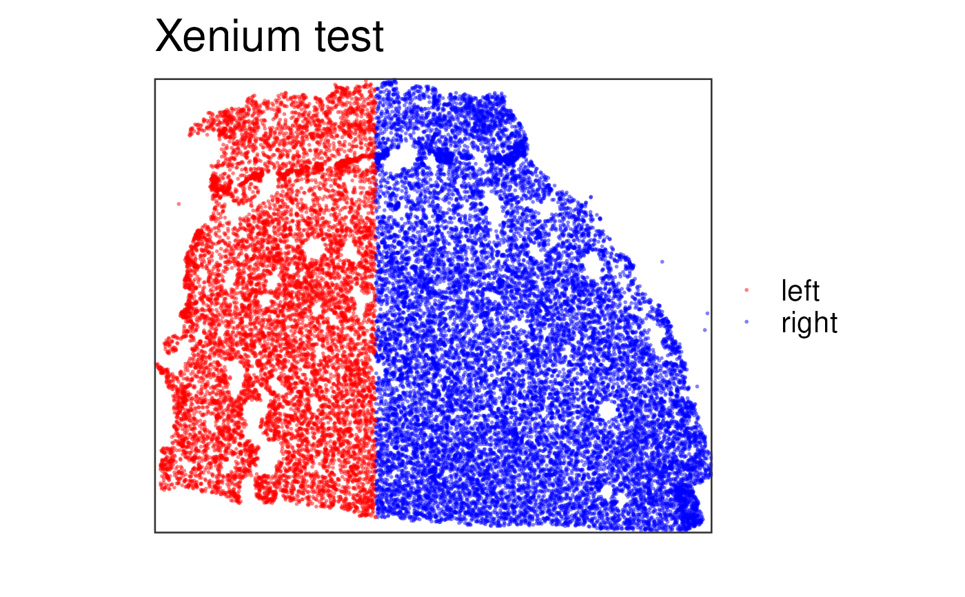
Sample spatial cluster visualization workhorse function for Xenium data with centroid based spatailCoords

This function visualizes clusters or categorical variables for one given sample at the cell-level. This is the function that does all the plotting behind vis_clus() when datatype = "Xenium". To visualize gene-level (or any continuous variable) use vis_gene_c().

vis_clus_c(
  spe,
  d,
  clustervar,
  sampleid = unique(spe$sample_id)[1],
  colors,
  title,
  alpha = NA,
  point_size = 1,
  auto_crop = TRUE,
  na_color = "#CCCCCC40"
)

Arguments

spe: A SpatialExperiment-class object. See fetch_data() for how to download some example objects or read10xVisiumWrapper() to read in spaceranger --count output files and build your own spe object.
d: A data.frame() with the sample-level information. This is typically obtained using cbind(colData(spe), spatialCoords(spe)).
clustervar: A character(1) with the name of the colData(spe) column that has the cluster values.
sampleid: A character(1) specifying which sample to plot from colData(spe)$sample_id (formerly colData(spe)$sample_name).
colors: A vector of colors to use for visualizing the clusters from clustervar. If the vector has names, then those should match the values of clustervar.
title: The title for the plot.
alpha: A numeric(1) in the [0, 1] range that specifies the transparency level of the data on the spots.
point_size: A numeric(1) specifying the size of the points. Defaults to 1.25. Some colors look better if you use 2 for instance.
auto_crop: A logical(1) indicating whether to automatically crop the image / plotting area, which is useful if the Visium capture area is not centered on the image and if the image is not a square.
na_color: A character(1) specifying a color for the NA values. If you set alpha = NA then it's best to set na_color to a color that has alpha blending already, which will make non-NA values pop up more and the NA values will show with a lighter color. This behavior is lost when alpha is set to a non-NA value.

Value

A ggplot2 object.

Examples


if (enough_ram()) {
    ## Obtain the necessary data
    if (!exists("spe_xenium")) spe_xenium <- fetch_data("spe_xenium_example")

    ## Prepare the data for the plotting function
    spe_sub <- spe_xenium[, spe_xenium$sample_id == "Br1039"]

    # summary(spatialCoords(spe_sub)[,"x_centroid"])
    # summary(spatialCoords(spe_sub)[,"y_centroid"])

    ## add catagorical variable
    spe_sub$x_half <- ifelse(spatialCoords(spe_sub)[,"x_centroid"] < 3088, "left", "right")
    table(spe_sub$x_half)

    p <- vis_clus_c(
        spe = spe_sub,
        d = as.data.frame(cbind(colData(spe_sub), SpatialExperiment::spatialCoords(spe_sub)), optional = TRUE),
        clustervar = "x_half",
        sampleid = "sample01.1",
        #colors = libd_layer_colors,
        colors = c(left = "red", right = "blue"),
        title = "Xenium test",
        point_size = 1,
        alpha = 0.5
    )
    print(p)

    ## Clean up
    rm(spe_sub)
}
#> 2026-09-28 14:55:33.34982 loading file /github/home/.cache/R/BiocFileCache/e2d6c76d1f9_spe_Xenium_test.rds%3Frlkey%3D0ql1pu5d9qe448sjmkh3ja3o8%26st%3Dnpwqxtdk%26dl%3D1

Sample spatial cluster visualization workhorse function for Xenium data with centroid based spatailCoords

Arguments

Value

See also

Examples