Get Started with DeconvoBuddies
Louise Huuki-Myers
Lieber Institute for Brain Development, Johns Hopkins Medical Campuslahuuki@gmail.com
31 March 2026
Source:vignettes/DeconvoBuddies.Rmd
DeconvoBuddies.RmdIntroduction
DeconvoBuddies is an R package developed to assist in
running bulk RNA-seq deconvolution. This package provides functions to
access a data set designed to evaluate deconvolution method performance,
find marker genes, and create plots useful in deconvolution.
This package is associated with “Benchmark of cellular deconvolution methods using a multi-assay reference dataset from postmortem human prefrontal cortex” from Huuki-Myers et al. (10.1101/2024.02.09.579665v2)[https://www.biorxiv.org/content/10.1101/2024.02.09.579665v2].
Basics
Install DeconvoBuddies
R is an open-source statistical environment which can be
easily modified to enhance its functionality via packages. DeconvoBuddies
is a R package available via the Bioconductor repository for packages.
R can be installed on any operating system from CRAN after which you can install
DeconvoBuddies
by using the following commands in your R session:
if (!requireNamespace("BiocManager", quietly = TRUE)) {
    install.packages("BiocManager")
}

BiocManager::install("DeconvoBuddies")

## Check that you have a valid Bioconductor installation
BiocManager::valid()
Required knowledge
DeconvoBuddies is based on many other packages and in particular in those that have implemented the infrastructure needed for dealing with snRNA-seq data. That is, packages like SingleCellExperiment.
If you are asking yourself the question “Where do I start using Bioconductor?” you might be interested in this blog post.
Asking for help
As package developers, we try to explain clearly how to use our
packages and in which order to use the functions. But R and
Bioconductor have a steep learning curve so it is critical
to learn where to ask for help. The blog post quoted above mentions some
but we would like to highlight the Bioconductor support site
as the main resource for getting help: remember to use the
DeconvoBuddies tag and check the older
posts. Other alternatives are available such as creating GitHub
issues and tweeting. However, please note that if you want to receive
help you should adhere to the posting
guidelines. It is particularly critical that you provide a small
reproducible example and your session information so package developers
can track down the source of the error.
Citing DeconvoBuddies
We hope that DeconvoBuddies will be useful for your research. Please use the following information to cite the package and the overall approach. Thank you!
## Citation info
citation("DeconvoBuddies")
#> To cite package 'DeconvoBuddies' in publications use:
#>
#>   Huuki-Myers LA, Maynard KR, Hicks SC, Zandi P, Kleinman JE, Hyde TM,
#>   Goes FS, Collado-Torres L (2026). _DeconvoBuddies: a R/Bioconductor
#>   package with deconvolution helper functions_.
#>   doi:10.18129/B9.bioc.DeconvoBuddies
#>   <https://doi.org/10.18129/B9.bioc.DeconvoBuddies>.
#>   https://github.com/LieberInstitute/DeconvoBuddies/DeconvoBuddies - R
#>   package version 1.3.2,
#>   <http://www.bioconductor.org/packages/DeconvoBuddies>.
#>
#>   Huuki-Myers LA, Montgomery KD, Kwon SH, Cinquemani S, Eagles NJ,
#>   Gonzalez-Padilla D, Maden SK, Kleinman JE, Hyde TM, Hicks SC, Maynard
#>   KR, Collado-Torres L (2025). "Benchmark of cellular deconvolution
#>   methods using a multi-assay dataset from postmortem human prefrontal
#>   cortex." _Genome Biol_. doi:10.1186/s13059-025-03552-3
#>   <https://doi.org/10.1186/s13059-025-03552-3>.
#>   <https://doi.org/10.1186/s13059-025-03552-3>.
#>
#> To see these entries in BibTeX format, use 'print(<citation>,
#> bibtex=TRUE)', 'toBibtex(.)', or set
#> 'options(citation.bibtex.max=999)'.
Quick start to using DeconvoBuddies
Let’s load some packages we’ll use in this vignette.
suppressMessages({
    library("DeconvoBuddies")
    library("SummarizedExperiment")
    library("dplyr")
    library("tidyr")
    library("tibble")
})
Access Data
Use fetch_deconvo_data to download RNA sequencing data
from the Human
DLPFC (Huuki-Myers, Montgomery, Kwon, Cinquemani, Eagles,
Gonzalez-Padilla, Maden, Kleinman, Hyde, Hicks, Maynard, and
Collado-Torres, 2025).
rse_gene: 110 samples of bulk RNA-seq. [110 bulk RNA-seq samples x 21k genes] (41 MB).sce: snRNA-seq data from the Human DLPFC. [77k nuclei x 36k genes] (172 MB)sce_DLPFC_example: Sub-set ofsceuseful for testing. [10k nuclei x 557 genes] (49 MB)
## Access and snRNA-seq example data
if (!exists("sce_DLPFC_example")) sce_DLPFC_example <- fetch_deconvo_data("sce_DLPFC_example")
#> 2026-03-31 18:34:17.672672 Access ExperimentHub EH9626
#> see ?DeconvoBuddies and browseVignettes('DeconvoBuddies') for documentation
#> loading from cache
#> require("SingleCellExperiment")

## Explore snRNA-seq data in sce_DLPFC_example
sce_DLPFC_example
#> class: SingleCellExperiment
#> dim: 557 10000
#> metadata(3): Samples cell_type_colors cell_type_colors_broad
#> assays(1): logcounts
#> rownames(557): GABRD PRDM16 ... AFF2 MAMLD1
#> rowData names(7): source type ... gene_type binomial_deviance
#> colnames(10000): 8_AGTGACTGTAGTTACC-1 17_GCAGCCAGTGAGTCAG-1 ...
#>   12_GGACGTCTCTGACAGT-1 1_GGTTAACTCTCTCTAA-1
#> colData names(32): Sample Barcode ... cellType_layer layer_annotation
#> reducedDimNames(0):
#> mainExpName: NULL
#> altExpNames(0):

## Access Bulk RNA-seq data
if (!exists("rse_gene")) rse_gene <- fetch_deconvo_data("rse_gene")
#> 2026-03-31 18:34:20.298668 Access ExperimentHub EH9625
#> see ?DeconvoBuddies and browseVignettes('DeconvoBuddies') for documentation
#> loading from cache

## Explore bulk data in rse_gene
rse_gene
#> class: RangedSummarizedExperiment
#> dim: 21745 110
#> metadata(1): SPEAQeasy_settings
#> assays(2): counts logcounts
#> rownames(21745): ENSG00000227232.5 ENSG00000278267.1 ...
#>   ENSG00000210195.2 ENSG00000210196.2
#> rowData names(11): Length gencodeID ... gencodeTx passExprsCut
#> colnames(110): 2107UNHS-0291_Br2720_Mid_Bulk
#>   2107UNHS-0291_Br2720_Mid_Cyto ... AN00000906_Br8667_Mid_Cyto
#>   AN00000906_Br8667_Mid_Nuc
#> colData names(80): SAMPLE_ID Sample ... diagnosis qc_class
For more details on this dataset, and an example deconvolution run check out the Vignette: Deconvolution Benchmark in Human DLPFC.
Marker Finding
Using MeanRatio to Find Cell Type Markers
Accurate deconvolution requires highly specific marker genes for each
cell type to be defined. To select genes specific for each cell type,
you can evaluate the MeanRatio for each gene x each cell type,
where
MeanRatio = mean(Expression of target cell type) / mean(Expression of highest non-target cell type).
These values can be calculated for a single cell RNA-seq dataset
using get_mean_ratio(). This can also work for
spatially-resolved transcriptomics datasets. That is,
get_mean_ratio() can also work with
SpatialExperiment::SpatialExperiment() objects.
## find marker genes with get_mean_ratio
marker_stats <- get_mean_ratio(
    sce_DLPFC_example,
    cellType_col = "cellType_broad_hc",
    gene_name = "gene_name",
    gene_ensembl = "gene_id"
)

## explore tibble output, gene with high MeanRatio values are good marker genes
marker_stats
#> # A tibble: 762 × 10
#>    gene       cellType.target mean.target cellType.2nd mean.2nd MeanRatio
#>    <chr>      <fct>                 <dbl> <fct>           <dbl>     <dbl>
#>  1 CD22       Oligo                  1.36 OPC            0.0730      18.6
#>  2 LINC01608  Oligo                  2.39 Micro          0.142       16.8
#>  3 FOLH1      Oligo                  1.59 OPC            0.101       15.7
#>  4 SLC5A11    Oligo                  2.14 Micro          0.145       14.7
#>  5 AC012494.1 Oligo                  2.42 OPC            0.169       14.3
#>  6 ST18       Oligo                  4.65 OPC            0.329       14.1
#>  7 MAG        Oligo                  1.44 Astro          0.103       14.0
#>  8 ANLN       Oligo                  1.60 Micro          0.115       13.9
#>  9 CLDN11     Oligo                  1.82 EndoMural      0.146       12.5
#> 10 MOG        Oligo                  2.06 OPC            0.185       11.1
#> # ℹ 752 more rows
#> # ℹ 4 more variables: MeanRatio.rank <int>, MeanRatio.anno <chr>,
#> #   gene_ensembl <chr>, gene_name <chr>
For more discussion of finding marker genes with
DeconvoBuddies check out the Vignette:
Finding Marker Genes with DeconvoBuddies.
Plotting Tools
Creating A Cell Type Color palette
As you work with single-cell data and deconvolution outputs, it is
very useful to establish a consistent color palette to use across
different plots. The function create_cell_colors() returns
a named vector of hex values, corresponding to the names of cell types.
This list is compatible with functions like
ggplot2::scale_color_manual().
There are three palettes to choose from to generate colors or users can provide their own color palette:
“classic” (default): classic set of 8 cell type colors from LIBD, checked for visability and color blind accessibility.
“gg”: Equi-distant hues, same process for selecting colors as
ggplot- no maximum number“tableau”: tableau20 color set - max 20 colors
test_cell_types <- c("cell_A", "cell_B", "cell_C", "cell_D", "cell_E")

## Preview "classic" colors
test_cell_colors_classic <- create_cell_colors(
    cell_types = test_cell_types,
    palette_name = "classic",
    preview = TRUE
)
#> Creating classic palette for 5 broad cell types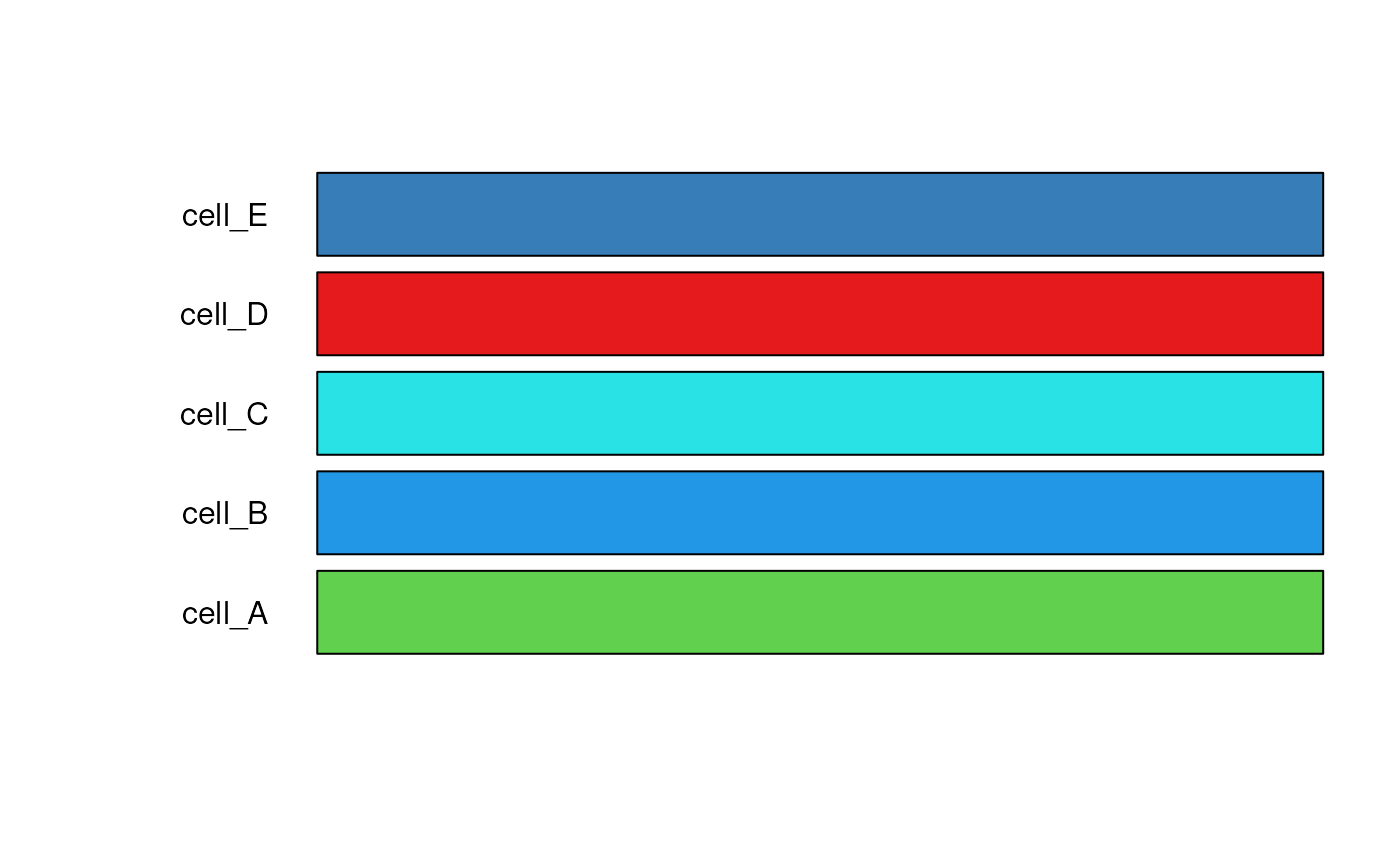
## Preview "gg" colors
test_cell_colors_gg <- create_cell_colors(
    cell_types = test_cell_types,
    palette_name = "gg",
    preview = TRUE
)
#> Creating gg palette for 5 broad cell types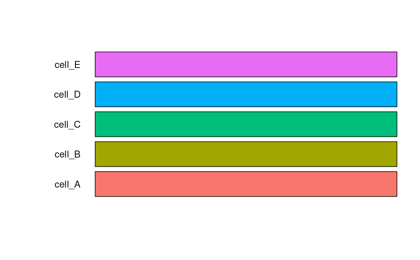
## Preview "tableau" colors
test_cell_colors_tableau <- create_cell_colors(
    cell_types = test_cell_types,
    palette_name = "tableau",
    preview = TRUE
)
#> Creating tableau palette for 5 broad cell types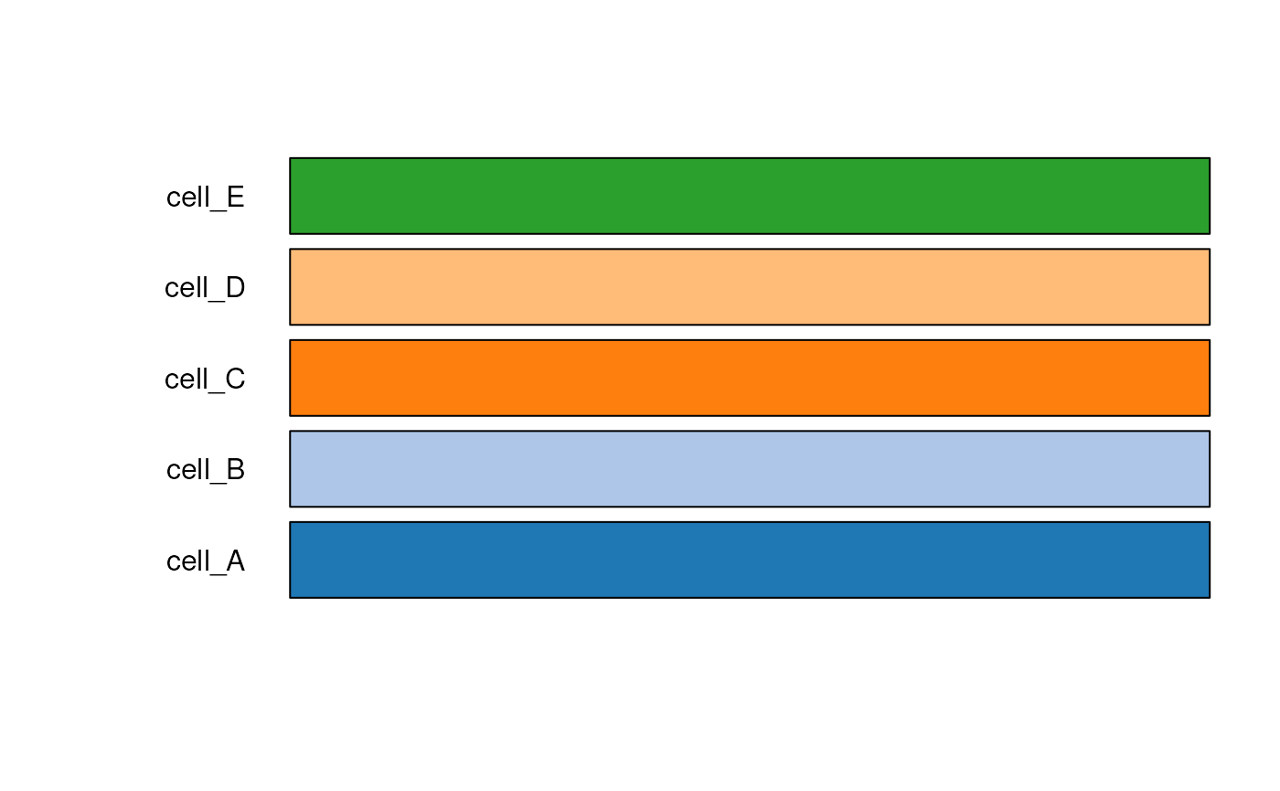
## Check the color hex codes for "tableau"
test_cell_colors_tableau
#>    cell_A    cell_B    cell_C    cell_D    cell_E
#> "#1F77B4" "#AEC7E8" "#FF7F0E" "#FFBB78" "#2CA02C"

## Provide a palette from RColorBrewer
test_cell_colors_brew <- create_cell_colors(
    cell_types = test_cell_types,
    palette = RColorBrewer::brewer.pal(n = length(test_cell_types), name = "Dark2"),
    preview = TRUE
)
#> Creating custom palette for 5 broad cell types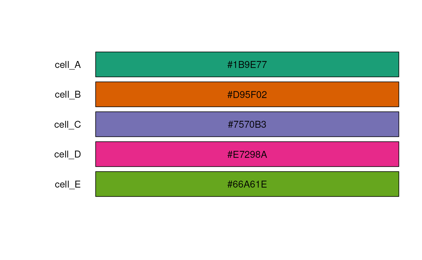
If there are sub-cell types with consistent delimiters, the
split argument creates a scale of related colors. This
helps expand on the maximum number of colors and makes your palette
flexible when considering different ‘resolutions’ of cell types. This
works by ignoring any prefixes after the split character.
In this example below, Excit_01 and Excit_02
will just be considered as Excit since
split = "_".
my_cell_types <- levels(sce_DLPFC_example$cellType_hc)
## Ignore any suffix after the "_" character by using the "split" argument
my_cell_colors <- create_cell_colors(
    cell_types = my_cell_types,
    palette_name = "classic",
    preview = TRUE,
    split = "_"
)
#> Creating classic palette for 8 broad cell types
#> Creating fine cell type gradients for 4 cell types
Plot Expression of Top Markers
The function plot_marker_express() helps quickly
visualize expression of top marker genes, by ordering and annotating
violin plots of expression over cell type. Here we’ll plot the
expression of the top 6 marker genes for Astrocytes.
# plot expression of the top 6 Astro marker genes
plot_marker_express(
    sce = sce_DLPFC_example,
    stats = marker_stats,
    cell_type = "Astro",
    n_genes = 6,
    cellType_col = "cellType_broad_hc",
    color_pal = my_cell_colors
)
#> Warning: No shared levels found between `names(values)` of the manual scale and the
#> data's fill values.
#> No shared levels found between `names(values)` of the manual scale and the
#> data's fill values.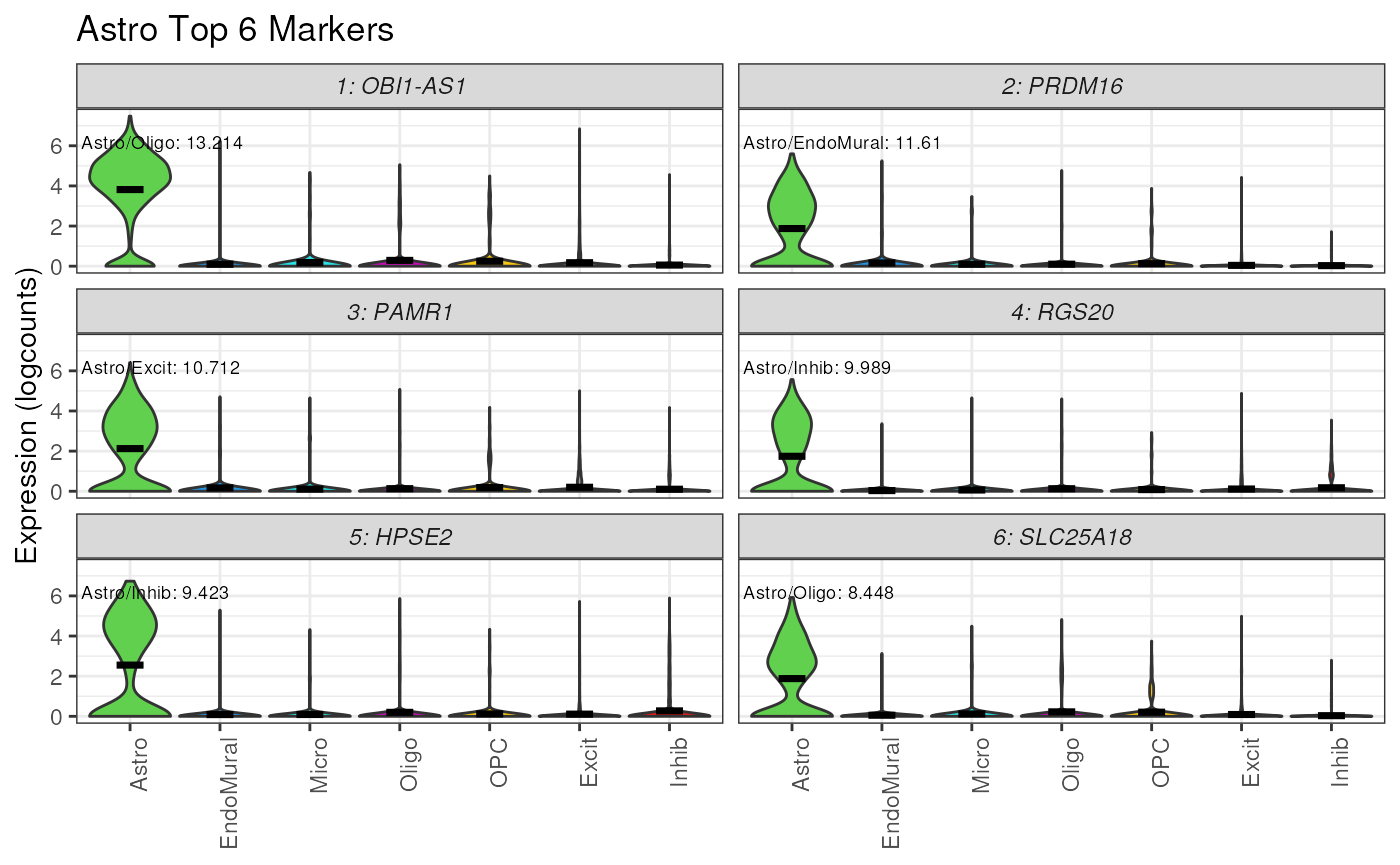
The violin plots of gene expression confirm the cell type specificity of these marker genes, most of the nuclei with high expression of these six genes are astrocytes (Astro).
Plot Composition Bar Plot
The output of deconvolution are cell type estimates that sum to 1. A
good visulization for these predictions is a stacked bar plot. The
function plot_composition_bar() creates a stacked bar plot
showing the cell type proportion for each sample, or the average
proportion for a group of samples. In this example data, the
RNum is a sample (donor) identifier and Dx is
a group variable for the diagnosis status of the donors.
# load example data
data("rse_bulk_test")
data("est_prop_test")

# access the colData of a test rse dataset
pd <- colData(rse_bulk_test) |>
    as.data.frame()

## pivot data to long format and join with test estimated proportion data
est_prop_long <- est_prop_test |>
    rownames_to_column("RNum") |>
    pivot_longer(!RNum, names_to = "cell_type", values_to = "prop") |>
    left_join(pd)
#> Joining with `by = join_by(RNum)`

## explore est_prop_long
est_prop_long
#> # A tibble: 500 × 7
#>    RNum  cell_type    prop BrNum Sex   Dx        Age
#>    <chr> <chr>       <dbl> <chr> <chr> <chr>   <dbl>
#>  1 R913  cell_A    0.431   Br001 F     Case     71.9
#>  2 R913  cell_B    0.242   Br001 F     Case     71.9
#>  3 R913  cell_C    0.110   Br001 F     Case     71.9
#>  4 R913  cell_D    0.174   Br001 F     Case     71.9
#>  5 R913  cell_E    0.0426  Br001 F     Case     71.9
#>  6 R602  cell_A    0.286   Br002 F     Control  73.1
#>  7 R602  cell_B    0.392   Br002 F     Control  73.1
#>  8 R602  cell_C    0.207   Br002 F     Control  73.1
#>  9 R602  cell_D    0.00186 Br002 F     Control  73.1
#> 10 R602  cell_E    0.113   Br002 F     Control  73.1
#> # ℹ 490 more rows

## the composition bar plot shows cell type composition for Sample
plot_composition_bar(est_prop_long,
    x_col = "RNum",
    add_text = FALSE
) +
    ggplot2::scale_fill_manual(values = test_cell_colors_classic)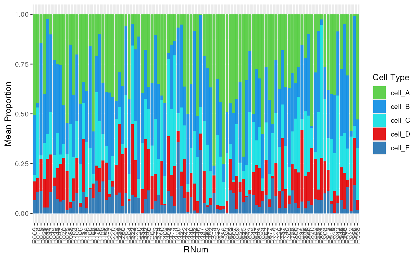
## the composition bar plot shows the average cell type composition for each Dx
plot_composition_bar(est_prop_long, x_col = "Dx") +
    ggplot2::scale_fill_manual(values = test_cell_colors_classic)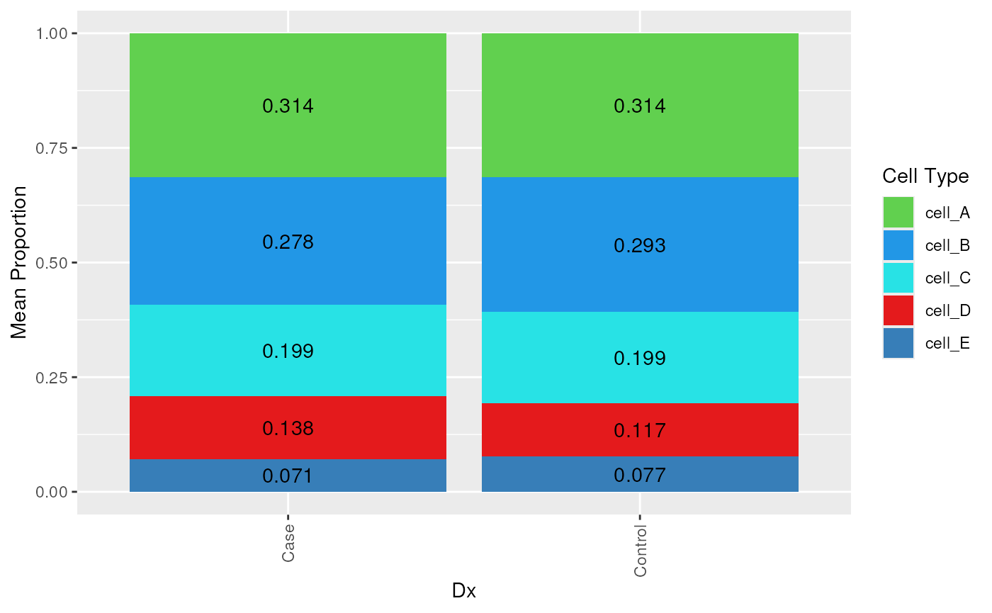
We can see that the mean proportions of cell types A through E are
very similar across the Dx groups (Case and
Control). In this case, this is expected given that we are
using simulated data. Although if you look across each donor with
RNum we can see more variability across the simulated
data.
Since you are now familiar with the basic overview of
DeconvoBuddies, you are now ready to dive deeper into:
- the selection of marker genes,
- followed by the application of
DeconvoBuddiesto the Human Brain (DLPFC) Deconvolution dataset.
Reproducibility
The DeconvoBuddies package (Huuki-Myers, Maynard, Hicks, Zandi, Kleinman, Hyde, Goes, and Collado-Torres, 2026) was made possible thanks to:
- R (R Core Team, 2026)
- AnnotationHub (Morgan and Shepherd, 2025)
- BiocFileCache (Shepherd and Morgan, 2025)
- DelayedMatrixStats (Hickey, 2025)
- dplyr (Wickham, François, Henry, Müller, and Vaughan, 2026)
- ExperimentHub (Morgan and Shepherd, 2025)
- ggplot2 (Wickham, 2016)
- graphics (R Core Team, 2026)
- grDevices (R Core Team, 2026)
- MatrixGenerics (Ahlmann-Eltze, Hickey, and Pagès, 2025)
- methods (R Core Team, 2026)
- purrr (Wickham and Henry, 2026)
- rafalib (Irizarry and Love, 2025)
- reshape2 (Wickham, 2007)
- S4Vectors (Pagès, Lawrence, and Aboyoun, 2025)
- scran (Lun, McCarthy, and Marioni, 2016)
- SingleCellExperiment (Amezquita, Lun, Becht, Carey, Carpp, Geistlinger, Marini, Rue-Albrecht, Risso, Soneson, Waldron, Pages, Smith, Huber, Morgan, Gottardo, and Hicks, 2020)
- spatialLIBD (Pardo, Spangler, Weber, Hicks, Jaffe, Martinowich, Maynard, and Collado-Torres, 2022)
- stats (R Core Team, 2026)
- stringr (Wickham, 2025)
- SummarizedExperiment (Morgan, Obenchain, Hester, and Pagès, 2026)
- tibble (Müller and Wickham, 2026)
- utils (R Core Team, 2026)
This vignette was generated using BiocStyle (Oleś, 2025) with knitr (Xie, 2025) and rmarkdown (Allaire, Xie, Dervieux, McPherson, Luraschi, Ushey, Atkins, Wickham, Cheng, Chang, and Iannone, 2026) running behind the scenes.
Citations made with RefManageR (McLean, 2017).
This package was developed using biocthis.
R session information.
#> ─ Session info ───────────────────────────────────────────────────────────────────────────────────────────────────────
#>  setting  value
#>  version  R Under development (unstable) (2026-03-28 r89738)
#>  os       Ubuntu 24.04.4 LTS
#>  system   x86_64, linux-gnu
#>  ui       X11
#>  language en
#>  collate  en_US.UTF-8
#>  ctype    en_US.UTF-8
#>  tz       UTC
#>  date     2026-03-31
#>  pandoc   3.9.0.2 @ /usr/bin/ (via rmarkdown)
#>  quarto   1.8.25 @ /usr/local/bin/quarto
#>
#> ─ Packages ───────────────────────────────────────────────────────────────────────────────────────────────────────────
#>  package              * version    date (UTC) lib source
#>  abind                  1.4-8      2024-09-12 [1] CRAN (R 4.6.0)
#>  AnnotationDbi          1.73.0     2025-10-31 [1] Bioconductor 3.23 (R 4.6.0)
#>  AnnotationHub          4.1.0      2025-10-31 [1] Bioconductor 3.23 (R 4.6.0)
#>  attempt                0.3.1      2020-05-03 [1] CRAN (R 4.6.0)
#>  backports              1.5.0      2024-05-23 [1] CRAN (R 4.6.0)
#>  beachmat               2.27.3     2026-02-27 [1] Bioconductor 3.23 (R 4.7.0)
#>  beeswarm               0.4.0      2021-06-01 [1] CRAN (R 4.6.0)
#>  benchmarkme            1.0.8      2022-06-12 [1] CRAN (R 4.6.0)
#>  benchmarkmeData        2.0.0      2026-01-19 [1] CRAN (R 4.6.0)
#>  bibtex                 0.5.2      2026-02-03 [1] CRAN (R 4.6.0)
#>  Biobase              * 2.71.0     2025-10-30 [1] Bioconductor 3.23 (R 4.6.0)
#>  BiocFileCache          3.1.0      2025-10-30 [1] Bioconductor 3.23 (R 4.6.0)
#>  BiocGenerics         * 0.57.0     2025-10-30 [1] Bioconductor 3.23 (R 4.6.0)
#>  BiocIO                 1.21.0     2025-10-30 [1] Bioconductor 3.23 (R 4.6.0)
#>  BiocManager            1.30.27    2025-11-14 [2] CRAN (R 4.7.0)
#>  BiocNeighbors          2.5.4      2026-02-12 [1] Bioconductor 3.23 (R 4.7.0)
#>  BiocParallel           1.45.0     2025-10-30 [1] Bioconductor 3.23 (R 4.6.0)
#>  BiocSingular           1.27.1     2025-11-17 [1] Bioconductor 3.23 (R 4.6.0)
#>  BiocStyle            * 2.39.0     2025-10-30 [1] Bioconductor 3.23 (R 4.6.0)
#>  BiocVersion            3.23.1     2025-10-30 [2] Bioconductor 3.23 (R 4.7.0)
#>  Biostrings             2.79.5     2026-03-06 [1] Bioconductor 3.23 (R 4.7.0)
#>  bit                    4.6.0      2025-03-06 [1] CRAN (R 4.6.0)
#>  bit64                  4.6.0-1    2025-01-16 [1] CRAN (R 4.6.0)
#>  bitops                 1.0-9      2024-10-03 [1] CRAN (R 4.6.0)
#>  blob                   1.3.0      2026-01-14 [1] CRAN (R 4.6.0)
#>  bluster                1.21.1     2026-03-05 [1] Bioconductor 3.23 (R 4.7.0)
#>  bookdown               0.46       2025-12-05 [1] CRAN (R 4.6.0)
#>  bslib                  0.10.0     2026-01-26 [2] CRAN (R 4.7.0)
#>  cachem                 1.1.0      2024-05-16 [2] CRAN (R 4.7.0)
#>  cigarillo              1.1.0      2025-10-31 [1] Bioconductor 3.23 (R 4.6.0)
#>  circlize               0.4.17     2025-12-08 [1] CRAN (R 4.6.0)
#>  cli                    3.6.5      2025-04-23 [2] CRAN (R 4.7.0)
#>  clue                   0.3-68     2026-03-26 [1] CRAN (R 4.7.0)
#>  cluster                2.1.8.2    2026-02-05 [3] CRAN (R 4.7.0)
#>  codetools              0.2-20     2024-03-31 [3] CRAN (R 4.7.0)
#>  colorspace             2.1-2      2025-09-22 [1] CRAN (R 4.6.0)
#>  ComplexHeatmap         2.27.1     2026-01-30 [1] Bioconductor 3.23 (R 4.6.0)
#>  config                 0.3.2      2023-08-30 [1] CRAN (R 4.6.0)
#>  cowplot                1.2.0      2025-07-07 [1] CRAN (R 4.6.0)
#>  crayon                 1.5.3      2024-06-20 [2] CRAN (R 4.7.0)
#>  curl                   7.0.0      2025-08-19 [2] CRAN (R 4.7.0)
#>  data.table             1.18.2.1   2026-01-27 [1] CRAN (R 4.6.0)
#>  DBI                    1.3.0      2026-02-25 [1] CRAN (R 4.7.0)
#>  dbplyr                 2.5.2      2026-02-13 [1] CRAN (R 4.7.0)
#>  DeconvoBuddies       * 1.3.2      2026-03-31 [1] Bioconductor
#>  DelayedArray           0.37.0     2025-10-31 [1] Bioconductor 3.23 (R 4.6.0)
#>  DelayedMatrixStats     1.33.0     2025-10-31 [1] Bioconductor 3.23 (R 4.6.0)
#>  desc                   1.4.3      2023-12-10 [2] CRAN (R 4.7.0)
#>  digest                 0.6.39     2025-11-19 [2] CRAN (R 4.7.0)
#>  doParallel             1.0.17     2022-02-07 [1] CRAN (R 4.6.0)
#>  dplyr                * 1.2.0      2026-02-03 [1] CRAN (R 4.6.0)
#>  dqrng                  0.4.1      2024-05-28 [1] CRAN (R 4.6.0)
#>  DT                     0.34.0     2025-09-02 [1] CRAN (R 4.6.0)
#>  edgeR                  4.9.4      2026-03-02 [1] Bioconductor 3.23 (R 4.7.0)
#>  evaluate               1.0.5      2025-08-27 [2] CRAN (R 4.7.0)
#>  ExperimentHub          3.1.0      2025-10-31 [1] Bioconductor 3.23 (R 4.6.0)
#>  farver                 2.1.2      2024-05-13 [1] CRAN (R 4.6.0)
#>  fastmap                1.2.0      2024-05-15 [2] CRAN (R 4.7.0)
#>  filelock               1.0.3      2023-12-11 [1] CRAN (R 4.6.0)
#>  foreach                1.5.2      2022-02-02 [1] CRAN (R 4.6.0)
#>  fs                     2.0.1      2026-03-24 [2] CRAN (R 4.7.0)
#>  generics             * 0.1.4      2025-05-09 [1] CRAN (R 4.6.0)
#>  GenomicAlignments      1.47.0     2025-10-31 [1] Bioconductor 3.23 (R 4.6.0)
#>  GenomicRanges        * 1.63.1     2025-12-08 [1] Bioconductor 3.23 (R 4.6.0)
#>  GetoptLong             1.1.0      2025-11-28 [1] CRAN (R 4.6.0)
#>  ggbeeswarm             0.7.3      2025-11-29 [1] CRAN (R 4.6.0)
#>  ggplot2                4.0.2      2026-02-03 [1] CRAN (R 4.6.0)
#>  ggrepel                0.9.8      2026-03-17 [1] CRAN (R 4.7.0)
#>  GlobalOptions          0.1.3      2025-11-28 [1] CRAN (R 4.6.0)
#>  glue                   1.8.0      2024-09-30 [2] CRAN (R 4.7.0)
#>  golem                  0.5.1      2024-08-27 [1] CRAN (R 4.6.0)
#>  gridExtra              2.3        2017-09-09 [1] CRAN (R 4.6.0)
#>  gtable                 0.3.6      2024-10-25 [1] CRAN (R 4.6.0)
#>  htmltools              0.5.9      2025-12-04 [2] CRAN (R 4.7.0)
#>  htmlwidgets            1.6.4      2023-12-06 [2] CRAN (R 4.7.0)
#>  httpuv                 1.6.17     2026-03-18 [2] CRAN (R 4.7.0)
#>  httr                   1.4.8      2026-02-13 [1] CRAN (R 4.7.0)
#>  httr2                  1.2.2      2025-12-08 [2] CRAN (R 4.7.0)
#>  igraph                 2.2.2      2026-02-12 [1] CRAN (R 4.7.0)
#>  IRanges              * 2.45.0     2025-10-31 [1] Bioconductor 3.23 (R 4.6.0)
#>  irlba                  2.3.7      2026-01-30 [1] CRAN (R 4.6.0)
#>  iterators              1.0.14     2022-02-05 [1] CRAN (R 4.6.0)
#>  jquerylib              0.1.4      2021-04-26 [2] CRAN (R 4.7.0)
#>  jsonlite               2.0.0      2025-03-27 [2] CRAN (R 4.7.0)
#>  KEGGREST               1.51.1     2025-11-17 [1] Bioconductor 3.23 (R 4.6.0)
#>  knitr                  1.51       2025-12-20 [2] CRAN (R 4.7.0)
#>  labeling               0.4.3      2023-08-29 [1] CRAN (R 4.6.0)
#>  later                  1.4.8      2026-03-05 [2] CRAN (R 4.7.0)
#>  lattice                0.22-9     2026-02-09 [3] CRAN (R 4.7.0)
#>  lazyeval               0.2.2      2019-03-15 [1] CRAN (R 4.6.0)
#>  lifecycle              1.0.5      2026-01-08 [2] CRAN (R 4.7.0)
#>  limma                  3.67.0     2025-10-30 [1] Bioconductor 3.23 (R 4.6.0)
#>  locfit                 1.5-9.12   2025-03-05 [1] CRAN (R 4.6.0)
#>  lubridate              1.9.5      2026-02-04 [1] CRAN (R 4.6.0)
#>  magick                 2.9.1      2026-02-28 [1] CRAN (R 4.7.0)
#>  magrittr               2.0.4      2025-09-12 [2] CRAN (R 4.7.0)
#>  Matrix                 1.7-5      2026-03-21 [3] CRAN (R 4.7.0)
#>  MatrixGenerics       * 1.23.0     2025-10-30 [1] Bioconductor 3.23 (R 4.6.0)
#>  matrixStats          * 1.5.0      2025-01-07 [1] CRAN (R 4.6.0)
#>  memoise                2.0.1      2021-11-26 [2] CRAN (R 4.7.0)
#>  metapod                1.19.2     2026-02-18 [1] Bioconductor 3.23 (R 4.7.0)
#>  mime                   0.13       2025-03-17 [2] CRAN (R 4.7.0)
#>  otel                   0.2.0      2025-08-29 [2] CRAN (R 4.7.0)
#>  paletteer              1.7.0      2026-01-08 [1] CRAN (R 4.6.0)
#>  pillar                 1.11.1     2025-09-17 [2] CRAN (R 4.7.0)
#>  pkgconfig              2.0.3      2019-09-22 [2] CRAN (R 4.7.0)
#>  pkgdown                2.2.0.9000 2026-03-31 [1] Github (r-lib/pkgdown@a6abe43)
#>  plotly                 4.12.0     2026-01-24 [1] CRAN (R 4.6.0)
#>  plyr                   1.8.9      2023-10-02 [1] CRAN (R 4.6.0)
#>  png                    0.1-9      2026-03-15 [1] CRAN (R 4.7.0)
#>  promises               1.5.0      2025-11-01 [2] CRAN (R 4.7.0)
#>  purrr                  1.2.1      2026-01-09 [2] CRAN (R 4.7.0)
#>  R6                     2.6.1      2025-02-15 [2] CRAN (R 4.7.0)
#>  rafalib                1.0.4      2025-04-08 [1] CRAN (R 4.6.0)
#>  ragg                   1.5.2      2026-03-23 [2] CRAN (R 4.7.0)
#>  rappdirs               0.3.4      2026-01-17 [2] CRAN (R 4.7.0)
#>  RColorBrewer           1.1-3      2022-04-03 [1] CRAN (R 4.6.0)
#>  Rcpp                   1.1.1      2026-01-10 [2] CRAN (R 4.7.0)
#>  RCurl                  1.98-1.18  2026-03-21 [1] CRAN (R 4.7.0)
#>  RefManageR           * 1.4.0      2022-09-30 [1] CRAN (R 4.6.0)
#>  rematch2               2.1.2      2020-05-01 [1] CRAN (R 4.6.0)
#>  reshape2               1.4.5      2025-11-12 [1] CRAN (R 4.6.0)
#>  restfulr               0.0.16     2025-06-27 [1] CRAN (R 4.6.0)
#>  rjson                  0.2.23     2024-09-16 [1] CRAN (R 4.6.0)
#>  rlang                  1.1.7      2026-01-09 [2] CRAN (R 4.7.0)
#>  rmarkdown              2.31       2026-03-26 [2] CRAN (R 4.7.0)
#>  Rsamtools              2.27.1     2026-03-08 [1] Bioconductor 3.23 (R 4.7.0)
#>  RSQLite                2.4.6      2026-02-06 [1] CRAN (R 4.6.0)
#>  rsvd                   1.0.5      2021-04-16 [1] CRAN (R 4.6.0)
#>  rtracklayer            1.71.3     2025-12-14 [1] Bioconductor 3.23 (R 4.6.0)
#>  S4Arrays               1.11.1     2025-11-25 [1] Bioconductor 3.23 (R 4.6.0)
#>  S4Vectors            * 0.49.0     2025-10-30 [1] Bioconductor 3.23 (R 4.6.0)
#>  S7                     0.2.1      2025-11-14 [1] CRAN (R 4.6.0)
#>  sass                   0.4.10     2025-04-11 [2] CRAN (R 4.7.0)
#>  ScaledMatrix           1.19.0     2025-10-31 [1] Bioconductor 3.23 (R 4.6.0)
#>  scales                 1.4.0      2025-04-24 [1] CRAN (R 4.6.0)
#>  scater                 1.39.3     2026-03-20 [1] Bioconductor 3.23 (R 4.7.0)
#>  scran                  1.39.1     2026-02-25 [1] Bioconductor 3.23 (R 4.7.0)
#>  scuttle                1.21.0     2025-11-03 [1] Bioconductor 3.23 (R 4.6.0)
#>  Seqinfo              * 1.1.0      2025-10-31 [1] Bioconductor 3.23 (R 4.6.0)
#>  sessioninfo          * 1.2.3      2025-02-05 [2] CRAN (R 4.7.0)
#>  shape                  1.4.6.1    2024-02-23 [1] CRAN (R 4.6.0)
#>  shiny                  1.13.0     2026-02-20 [2] CRAN (R 4.7.0)
#>  shinyWidgets           0.9.1      2026-03-09 [1] CRAN (R 4.7.0)
#>  SingleCellExperiment * 1.33.2     2026-03-24 [1] Bioconductor 3.23 (R 4.7.0)
#>  SparseArray            1.11.12    2026-03-30 [1] Bioconductor 3.23 (R 4.7.0)
#>  sparseMatrixStats      1.23.0     2025-10-30 [1] Bioconductor 3.23 (R 4.6.0)
#>  SpatialExperiment      1.21.0     2025-11-03 [1] Bioconductor 3.23 (R 4.6.0)
#>  spatialLIBD            1.23.2     2026-01-13 [1] Bioconductor 3.23 (R 4.6.0)
#>  statmod                1.5.1      2025-10-09 [1] CRAN (R 4.6.0)
#>  stringi                1.8.7      2025-03-27 [2] CRAN (R 4.7.0)
#>  stringr                1.6.0      2025-11-04 [2] CRAN (R 4.7.0)
#>  SummarizedExperiment * 1.41.1     2026-02-06 [1] Bioconductor 3.23 (R 4.6.0)
#>  systemfonts            1.3.2      2026-03-05 [2] CRAN (R 4.7.0)
#>  textshaping            1.0.5      2026-03-06 [2] CRAN (R 4.7.0)
#>  tibble               * 3.3.1      2026-01-11 [2] CRAN (R 4.7.0)
#>  tidyr                * 1.3.2      2025-12-19 [1] CRAN (R 4.6.0)
#>  tidyselect             1.2.1      2024-03-11 [1] CRAN (R 4.6.0)
#>  timechange             0.4.0      2026-01-29 [1] CRAN (R 4.6.0)
#>  utf8                   1.2.6      2025-06-08 [2] CRAN (R 4.7.0)
#>  vctrs                  0.7.2      2026-03-21 [2] CRAN (R 4.7.0)
#>  vipor                  0.4.7      2023-12-18 [1] CRAN (R 4.6.0)
#>  viridis                0.6.5      2024-01-29 [1] CRAN (R 4.6.0)
#>  viridisLite            0.4.3      2026-02-04 [1] CRAN (R 4.6.0)
#>  withr                  3.0.2      2024-10-28 [2] CRAN (R 4.7.0)
#>  xfun                   0.57       2026-03-20 [2] CRAN (R 4.7.0)
#>  XML                    3.99-0.23  2026-03-20 [1] CRAN (R 4.7.0)
#>  xml2                   1.5.2      2026-01-17 [2] CRAN (R 4.7.0)
#>  xtable                 1.8-8      2026-02-22 [2] CRAN (R 4.7.0)
#>  XVector                0.51.0     2025-10-31 [1] Bioconductor 3.23 (R 4.6.0)
#>  yaml                   2.3.12     2025-12-10 [2] CRAN (R 4.7.0)
#>
#>  [1] /__w/_temp/Library
#>  [2] /usr/local/lib/R/site-library
#>  [3] /usr/local/lib/R/library
#>  * ── Packages attached to the search path.
#>
#> ──────────────────────────────────────────────────────────────────────────────────────────────────────────────────────
Bibliography
[1] C. Ahlmann-Eltze, P. Hickey, and H. Pagès. MatrixGenerics: S4 Generic Summary Statistic Functions that Operate on Matrix-Like Objects. R package version 1.23.0. 2025. DOI: 10.18129/B9.bioc.MatrixGenerics. URL: https://bioconductor.org/packages/MatrixGenerics.
[2] J. Allaire, Y. Xie, C. Dervieux, et al. rmarkdown: Dynamic Documents for R. R package version 2.31. 2026. URL: https://github.com/rstudio/rmarkdown.
[3] R. Amezquita, A. Lun, E. Becht, et al. “Orchestrating single-cell analysis with Bioconductor”. In: Nature Methods 17 (2020), pp. 137–145. URL: https://www.nature.com/articles/s41592-019-0654-x.
[4] P. Hickey. DelayedMatrixStats: Functions that Apply to Rows and Columns of ‘DelayedMatrix’ Objects. R package version 1.33.0. 2025. DOI: 10.18129/B9.bioc.DelayedMatrixStats. URL: https://bioconductor.org/packages/DelayedMatrixStats.
[5] L. A. Huuki-Myers, K. R. Maynard, S. C. Hicks, et al. DeconvoBuddies: a R/Bioconductor package with deconvolution helper functions. https://github.com/LieberInstitute/DeconvoBuddies/DeconvoBuddies - R package version 1.3.2. 2026. DOI: 10.18129/B9.bioc.DeconvoBuddies. URL: http://www.bioconductor.org/packages/DeconvoBuddies.
[6] L. A. Huuki-Myers, K. D. Montgomery, S. H. Kwon, et al. “Benchmark of cellular deconvolution methods using a multi-assay dataset from postmortem human prefrontal cortex”. In: Genome Biol (2025). DOI: 10.1186/s13059-025-03552-3. URL: https://doi.org/10.1186/s13059-025-03552-3.
[7] R. A. Irizarry and M. I. Love. rafalib: Convenience Functions for Routine Data Exploration. R package version 1.0.4. 2025. DOI: 10.32614/CRAN.package.rafalib. URL: https://CRAN.R-project.org/package=rafalib.
[8] A. T. L. Lun, D. J. McCarthy, and J. C. Marioni. “A step-by-step workflow for low-level analysis of single-cell RNA-seq data with Bioconductor”. In: F1000Res. 5 (2016), p. 2122. DOI: 10.12688/f1000research.9501.2.
[9] M. W. McLean. “RefManageR: Import and Manage BibTeX and BibLaTeX References in R”. In: The Journal of Open Source Software (2017). DOI: 10.21105/joss.00338.
[10] M. Morgan, V. Obenchain, J. Hester, et al. SummarizedExperiment: A container (S4 class) for matrix-like assays. R package version 1.41.1. 2026. DOI: 10.18129/B9.bioc.SummarizedExperiment. URL: https://bioconductor.org/packages/SummarizedExperiment.
[11] M. Morgan and L. Shepherd. AnnotationHub: Client to access AnnotationHub resources. R package version 4.1.0. 2025. DOI: 10.18129/B9.bioc.AnnotationHub. URL: https://bioconductor.org/packages/AnnotationHub.
[12] M. Morgan and L. Shepherd. ExperimentHub: Client to access ExperimentHub resources. R package version 3.1.0. 2025. DOI: 10.18129/B9.bioc.ExperimentHub. URL: https://bioconductor.org/packages/ExperimentHub.
[13] K. Müller and H. Wickham. tibble: Simple Data Frames. R package version 3.3.1. 2026. DOI: 10.32614/CRAN.package.tibble. URL: https://CRAN.R-project.org/package=tibble.
[14] A. Oleś. BiocStyle: Standard styles for vignettes and other Bioconductor documents. R package version 2.39.0. 2025. DOI: 10.18129/B9.bioc.BiocStyle. URL: https://bioconductor.org/packages/BiocStyle.
[15] H. Pagès, M. Lawrence, and P. Aboyoun. S4Vectors: Foundation of vector-like and list-like containers in Bioconductor. R package version 0.49.0. 2025. DOI: 10.18129/B9.bioc.S4Vectors. URL: https://bioconductor.org/packages/S4Vectors.
[16] B. Pardo, A. Spangler, L. M. Weber, et al. “spatialLIBD: an R/Bioconductor package to visualize spatially-resolved transcriptomics data”. In: BMC Genomics (2022). DOI: 10.1186/s12864-022-08601-w. URL: https://doi.org/10.1186/s12864-022-08601-w.
[17] R Core Team. R: A Language and Environment for Statistical Computing. R Foundation for Statistical Computing (ROR: <https://ror.org/05qewa988>;). Vienna, Austria, 2026. DOI: 10.32614/R.manuals. URL: https://www.R-project.org/.
[18] L. Shepherd and M. Morgan. BiocFileCache: Manage Files Across Sessions. R package version 3.1.0. 2025. DOI: 10.18129/B9.bioc.BiocFileCache. URL: https://bioconductor.org/packages/BiocFileCache.
[19] H. Wickham. ggplot2: Elegant Graphics for Data Analysis. Springer-Verlag New York, 2016. ISBN: 978-3-319-24277-4. URL: https://ggplot2.tidyverse.org.
[20] H. Wickham. “Reshaping Data with the reshape Package”. In: Journal of Statistical Software 21.12 (2007), pp. 1–20. URL: https://www.jstatsoft.org/v21/i12/.
[21] H. Wickham. stringr: Simple, Consistent Wrappers for Common String Operations. R package version 1.6.0. 2025. DOI: 10.32614/CRAN.package.stringr. URL: https://CRAN.R-project.org/package=stringr.
[22] H. Wickham, R. François, L. Henry, et al. dplyr: A Grammar of Data Manipulation. R package version 1.2.0. 2026. DOI: 10.32614/CRAN.package.dplyr. URL: https://CRAN.R-project.org/package=dplyr.
[23] H. Wickham and L. Henry. purrr: Functional Programming Tools. R package version 1.2.1. 2026. DOI: 10.32614/CRAN.package.purrr. URL: https://CRAN.R-project.org/package=purrr.
[24] Y. Xie. knitr: A General-Purpose Package for Dynamic Report Generation in R. R package version 1.51. 2025. URL: https://yihui.org/knitr/.